Simultaneous Total Derivative Coloring For Separable Problems

When OpenMDAO solves for total derivatives, it loops over either design variables in ‘fwd’ mode or responses in ‘rev’ mode. For each of those variables, it performs a linear solve for each member of that variable, so for a scalar variable there would be only a single linear solve, and there would be N solves for an array variable of size N.

Certain problems have a special kind of sparsity structure in the total derivative Jacobian that allows OpenMDAO to solve for multiple derivatives simultaneously. This can result in far fewer linear solves and much-improved performance. These problems are said to have separable variables. The concept of separability is explained in the Theory Manual.

Simultaneous derivative coloring in OpenMDAO can be performed either statically or dynamically.

When mode is set to ‘fwd’ or ‘rev’, a unidirectional coloring algorithm is used to group columns or rows, respectively, for simultaneous derivative calculation. The algorithm used in this case is the greedy algorithm with ordering by incidence degree found in T. F. Coleman and J. J. More, Estimation of sparse Jacobian matrices and graph coloring problems, SIAM J. Numer. Anal., 20 (1983), pp. 187–209.

When using simultaneous derivatives, setting mode=’auto’ will indicate that bidirectional coloring should be used. Bidirectional coloring can significantly decrease the number of linear solves needed to generate the total Jacobian relative to coloring only in fwd or rev mode.

For more information on the bidirectional coloring algorithm, see T. F. Coleman and A. Verma, The efficient computation of sparse Jacobian matrices using automatic differentiation, SIAM J. Sci. Comput., 19 (1998), pp. 1210–1233.

Note

Bidirectional coloring is a new feature and should be considered experimental at this point.

The OpenMDAO algorithms use the sparsity patterns for the partial derivatives given by the declare_partials calls from all of the components in your model. So you should specify the sparsity of the partial derivatives of your components in order to make it possible to find a better automatic coloring.

Dynamic Coloring

Dynamic coloring computes the derivative colors at runtime, shortly after the driver begins the optimization. This has the advantage of simplicity and robustness to changes in the model, but adds the cost of the coloring computation to the run time of the optimization. Generally, however, this cost will be small relative to the cost of the full optimization unless your total jacobian is very large.

Activating dynamic coloring is simple. Just call the declare_coloring function on the driver. For example:

prob.driver.declare_coloring()

If you want to change the number of compute_totals calls that the coloring algorithm uses to compute the Jacobian sparsity (default is 3), the tolerance used to determine nonzeros (default is 1e-25), you can pass the num_full_jacs, and tol args. You can also pass the min_improve_pct arg, which specifies how much the coloring must reduce the number of linear solves required to generate the total Jacobian else coloring will be deactivated.

For example:

prob.driver.declare_coloring(num_full_jacs=2, tol=1e-20, min_improve_pct=10.)

If you want to perform a tolerance sweep, trying out a range of tolerances when determining what values of the sparsity matrix should be considered zero, then you can set the orders arg. OpenMDAO will then sweep over tolerances from the given tol plus and minus orders orders of magnitude. For each tolerance, it checks the number of nonzero values, and chooses a tolerance from the largest group of tolerances that share the same number of nonzeros. If it can’t find at least two tolerances that result in the same number of nonzeros, an exception is raised.

Here’s an example:

prob.driver.declare_coloring(tol=1e-35, orders=20)

Whenever a dynamic coloring is computed, the coloring is written to a file called total_coloring.pkl for later ‘static’ use. The file will be written in a directory specified in problem.options['coloring_dir']. If no value is set into problem.options['coloring_dir'] then the coloring_files directory under the current working directory at the time the problem is instantiated will be used.

You can see a more complete example of setting up an optimization with simultaneous derivatives in the Simple Optimization using Simultaneous Derivatives example.

Total coloring as a report

As part of the dynamic coloring process, OpenMDAO will automatically generate a visualization of the coloring that can be found in reports/{problem_name}/total_coloring.html. If the bokeh python plotting package is available, this report will be an interactive visualization, otherwise an ascii representation of the total coloring will be provided. More information about these visualizations is given below.

Static Coloring

To get rid of the runtime cost of computing the coloring, you can precompute it and tell the driver to use its precomputed coloring by calling the use_fixed_coloring method on the driver. Note that this call should be made after calling declare_coloring.

Driver.use_fixed_coloring(coloring=<object object>)

Tell the driver to use a precomputed coloring.

Parameters:

coloringstr or Coloring

A coloring filename or a Coloring object. If no arg is passed, filename will be determined automatically.

You don’t need to tell use_fixed_coloring the name of the coloring file to use, because it uses a fixed name, total_coloring.pkl, and knows what directory to look in based on the directory specified in problem.options['coloring_dir']. However, you can pass the name of a coloring file to use_fixed_coloring if you want to use a specific coloring file that doesn’t follow the standard naming convention.

While using a precomputed coloring has the advantage of removing the runtime cost of computing the coloring, it should be used with care, because any changes in the model, design variables, or responses can make the existing coloring invalid. If any configuration changes have been made to the optimization, it’s recommended to regenerate the coloring before re-running the optimization.

Updating total coloring from the command line

The total coloring can be regenerated and written to the total_coloring.pkl file in a directory determined by the value of problem.options['coloring_files'] using the following command:

openmdao total_coloring <your_script_name>

Note that if you have passed a coloring filename into use_fixed_coloring instead of letting the framework determine the filename automatically, the framework will not update the contents of the coloring file even if you run openmdao total_coloring from the command line.

The total_coloring command also generates summary information that can sometimes be useful. The tolerance that was actually used to determine if an entry in the total Jacobian is considered to be non-zero is displayed, along with the number of zero entries found in this case, and how many times that number of zero entries occurred when sweeping over different tolerances between +- a number of orders of magnitude around the given tolerance. If no tolerance is given, the default is 1e-15. If the number of occurrences is only 1, an exception will be raised, and you should increase the number of total derivative computations that the algorithm uses to compute the sparsity pattern. You can do that with the -n option. The following, for example, will perform the total derivative computation 5 times.

openmdao total_coloring <your_script_name> -n 5

Note that when multiple total jacobian computations are performed, we take the absolute values of each jacobian and add them together, then divide by the maximum value, resulting in values between 0 and 1 for each entry.

If repeating the total derivative computation multiple times doesn’t work, try changing the tolerance using the -t option as follows:

openmdao total_coloring <your_script_name> -n 5 -t 1e-10

Be careful when setting the tolerance, however, because if you make it too large then you may be zeroing out Jacobian entries that should not be ignored and your optimization may not converge.

If you want to examine the sparsity structure of your total Jacobian, you can use the –view option as follows:

openmdao total_coloring <your_script_name> --view

which will display a visualization of the sparsity structure with rows and columns labelled with the response and design variable names, respectively. See the figure here.

A text-based view is also available using the –textview arg. For example:

openmdao total_coloring <your_script_name> --textview

will display something like the following:

....................f 0  circle.area
f.........f.........f 1  r_con.g
.f.........f........f 2  r_con.g
..f.........f.......f 3  r_con.g
...f.........f......f 4  r_con.g
....f.........f.....f 5  r_con.g
.....f.........f....f 6  r_con.g
......f.........f...f 7  r_con.g
.......f.........f..f 8  r_con.g
........f.........f.f 9  r_con.g
.........f.........ff 10  r_con.g
f.........f.......... 11  theta_con.g
..f.........f........ 12  theta_con.g
....f.........f...... 13  theta_con.g
......f.........f.... 14  theta_con.g
........f.........f.. 15  theta_con.g
ff........ff......... 16  delta_theta_con.g
..ff........ff....... 17  delta_theta_con.g
....ff........ff..... 18  delta_theta_con.g
......ff........ff... 19  delta_theta_con.g
........ff........ff. 20  delta_theta_con.g
f.................... 21  l_conx.g
|indeps.x
          |indeps.y
                    |indeps.r

Note that the design variables are displayed along the bottom of the matrix, with a pipe symbol (|) that lines up with the starting column for that variable. Also, an ‘f’ indicates a nonzero value that is colored in ‘fwd’ mode, while an ‘r’ indicates a nonzero value colored in ‘rev’ mode. A ‘.’ indicates a zero value.

The coloring file will be written in pickle format to the standard location and will be loaded using the use_fixed_coloring function like this:

prob.driver.use_fixed_coloring()

Note that there are two ways to generate files that can be loaded using use_fixed_coloring. You can either run the openmdao total_coloring command line tool, or you can just run your model, and as long as you’ve called declare_coloring on your driver, it will automatically generate a coloring file that you can ‘lock in’ at some later point by adding a call to use_fixed_coloring, after you’re done making changes to your model.

Viewing total coloring from the command line

If you have a coloring file that was generated earlier and you want to view its statistics, you can use the openmdao view_coloring command to generate a small report.

openmdao view_coloring <your_coloring_file> -m

will show metadata associated with the creation of the coloring along with a short summary. For example:

Coloring metadata:
{'orders': 20, 'num_full_jacs': 3, 'tol': 1e-15}

Jacobian shape: (22, 21)  (13.42% nonzero)

FWD solves: 5   REV solves: 0

Total colors vs. total size: 5 vs 21  (76.2% improvement)

Time to compute sparsity: 0.024192 sec.
Time to compute coloring: 0.001076 sec.

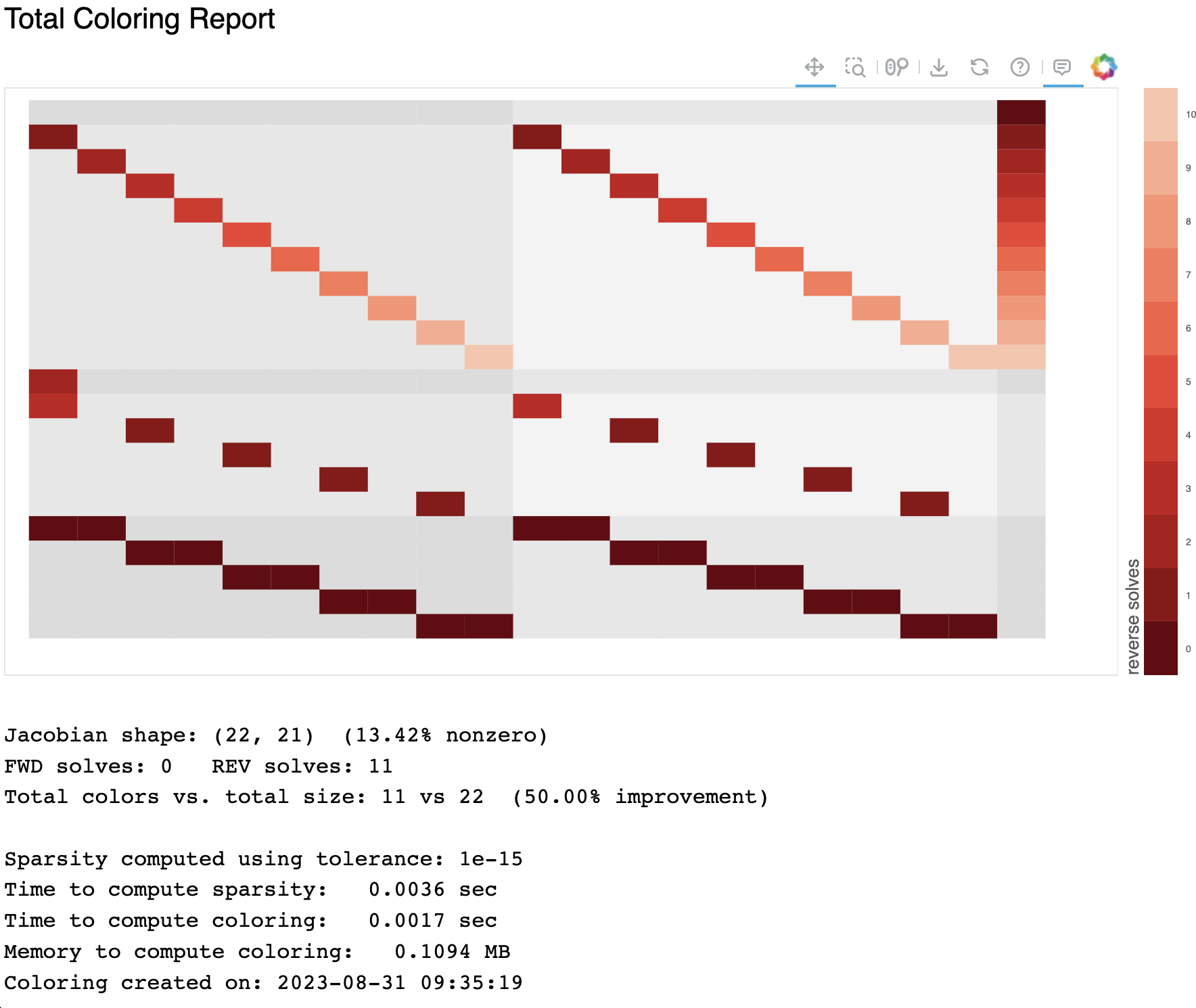
Adding a –view arg will pop up an interactive plot showing the coloring of the jacobian. Forward colors will be colored shades of blue and reverse colors will be colored in shades of red. Hovering over a particular cell of the Jacobian will display the location, the color number, the coloring direction, and the particular ‘of’ and ‘wrt’ variables for that particular sub-jacobian. Note that this viewer requires the installation of bokeh. See the figure below.

If bokeh is not available, then the resulting html viewer will contain an ascii version of the sparsity pattern similar to that in the previous section, along with some statistics about the coloring.

Note

Your coloring file(s) will be found in the standard directory problem.options[‘coloring_dir’]. That directory may contain a total coloring file, total_coloring.pkl, in additon to files containing partial derivative colorings for particular component classes or instances, as well as semi-total derivative coloring files for particular groups.

If you run openmdao total_coloring and it turns out there is no simultaneous total coloring available, or that you don’t gain very much by coloring, don’t be surprised. Not all total Jacobians are sparse enough to benefit significantly from simultaneous derivatives.

Viewing total coloring from a script

The openmdao.api includes a display_coloring function to allow viewing of coloring data from within a script. This function will generate an html file, but will render the coloring as plain text if bokeh is unavailable or if the as_text argument is True.

openmdao.utils.coloring.display_coloring(source, output_file='total_coloring.html', as_text=False, show=True, max_colors=200)

Display the coloring information from source to html format.

Parameters:

sourcestr or Coloring or Driver

The source of the coloring information. If given as a string, source should be a valid coloring file path. If given as a Driver, display_colroing will attempt to obtain coloring information from the Driver.

output_filestr or Path or None

The output file to which the coloring display should be sent. If as_text is True and output_file ends with .html, then the coloring will be sent to that file as html, otherwise it will the html file will be saved in a temporary file.

as_textbool

If True, render the coloring information using plain text.

showbool

If True, open the resulting html file in the system browser.

max_colorsint

Bokeh colormaps support at most 256 colors. Near the upper end of this interval, the colors are nearly white and may be difficult to distinguish. This setting sets the upper limit for the color index before the pattern repeats.

Checking that it works

After activating simultaneous derivatives, you should check your total derivatives using the check_totals function. The algorithm that we use still has a small chance of computing an incorrect coloring due to the possibility that the total Jacobian being analyzed by the algorithm contained one or more zero values that are only incidentally zero. Using check_totals is the way to be sure that something hasn’t gone wrong.

If you used the automatic coloring algorithm, and you find that check_totals is reporting incorrect total derivatives, then you should try using the -n and -t options mentioned earlier until you get the correct total derivatives.