Using OpenMDAO with MPI

In the feature notebooks for ParallelGroup and for Distributed Variables, you learned how to build a model that can take advantage of multiple processors to speed up your calculations. This document gives further details about how data is handled when using either of these features.

Parallel Subsystems

The ParallelGroup allows you to declare that a set of unconnected Components or Groups should be run in parallel. For example, consider the model in the following diagram:

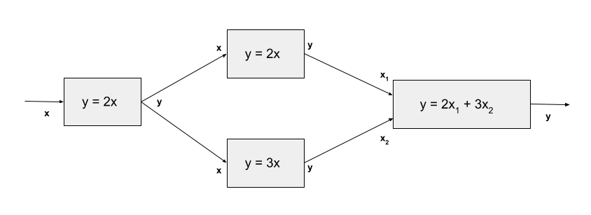
This model contains two components that don’t depend on each other’s outputs, and thus those calculations can be performed simultaneously by placing them in a ParallelGroup. When a model containing a ParallelGroup is run without using MPI, its components are just executed in succession. But when it is run using mpirun or mpiexec, its components are divided amongst the processes. To ensure that all subsystems execute in parallel, you should run with at least as many processes as there are subsystems. If you don’t provide enough processes, then some processes will sequentially execute some of the components. Some subsystems may require more processes than others. If you give your model more processes than are needed by the subsystems, those processes will be either be idle during execution of the parallel subsystem or will perform duplicate computations, depending upon how processes are assigned within a subsystem.

OpenMDAO can compute derivatives in forward or reverse mode, with the best choice of mode being determined by the ratio of the number of design variables vs. the number of responses. If the number of responses is greater than the number of design variables, then forward mode is best, and reverse is best if the number of design variables exceeds the number of responses. ‘Best’ in this case means requiring a smaller number of linear solves in order to compute the total jacobian matrix.

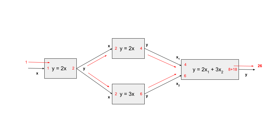
The following diagram shows forward mode derivative transfers for our example model running on 1 process.

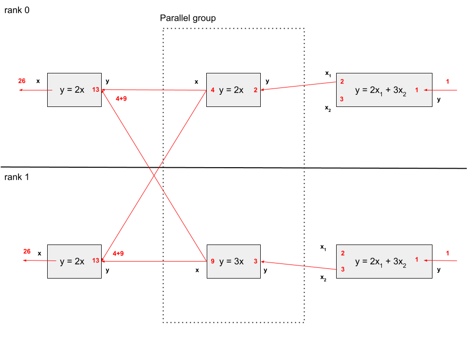
The next diagram shows the forward mode transfers for the same example executing on 2 processes. Note that the derivative values at the input and output of each component in the model are the same as they were in the 1 process case.

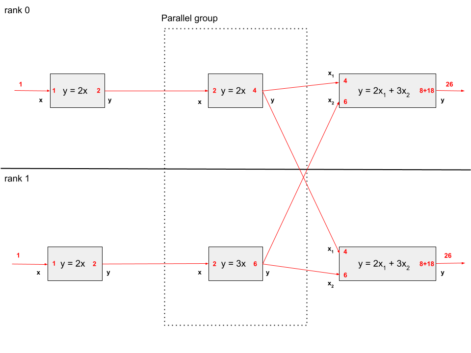
We see here that every component that isn’t under the ParallelGroup is executed on all processes. This is done to limit data transfer between the processes. Similarly, the input and output vectors on these components are the same on all processes. We sometimes call these duplicated variables, but it is clearer to call them non-parallel non-distributed variables.

In contrast, the inputs and outputs on the parallel components only exist on their execution processor(s). In this model, there are parallel outputs that need to be passed downstream to the final component. To make this happen, OpenMDAO scatters them from the rank(s) that contain them to the rank(s) that don’t. This can be seen in the diagram as the crossed arrows that connect to x1 and x2. Data transfers are done so as to minimize the amount of data passed between processes so, for example, the ‘y’ value from the duplicated ‘y=2x’ component, since it exists in both processes, is only passed to the connected ‘x’ input in the same process.

Since component execution is repeated on all processes, component authors need to be careful about file operations which can collide if they are called from all processes at once. The safest way to handle these is to restrict them to only write files on the root processor. In addition, the computation of derivatives is duplicated on all processes except for the components in the parallel group, which handle their own unique parts of the calculation.

Reverse-mode Derivatives in Parallel Subsystems

Reverse-mode derivative calculation uses different transfers than forward mode in order to ensure that the values of non-parallel non-distributed derivatives are consistent across processes and agree with derivatives from the same model if run in a single process.

The following diagram shows reverse mode derivative transfers for our example model running on 1 process.

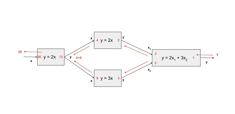
In this diagram, our model has one derivative to compute. We start with a seed of 1.0 in the output, and propagate that through the model (as denoted by the red arrows), multiplying by the sub-jacobians in each component as we go. Whenever we have an internal output that is connected to multiple inputs, we need to sum the contributions that are propagated there in reverse mode. The end result is the derivative across these components.

Now, let’s examine this process under MPI with 2 processors:

We see here, as in the forward case, the derivative values in the component inputs and outputs agree with those we saw in the non-parallel case. Note that, as mentioned above, we have to sum the values from multiple inputs if they are connected to the same output. However, when running on multiple processes, some of our inputs are duplicated, i.e. we have the same input existing in multiple processes. In that case, assuming the input is not distributed, we do not sum the multiple instances together but instead use only one of the values, either the value from the same process as the output if it exists, or the value from the lowest rank process where it does exist.

Distributed Components

OpenMDAO also allows you to add distributed variables to any implicit or explicit component. These can be refered to as distributed components, though there isn’t a distributed component class. This feature gives you the ability to parallelize the internal calculation of your component just like the ParallelGroup can parallelize a larger part of the model. Distributed variables hold different values on all processors, and can even be empty on some processors if declared as such. Components containing mixed distributed/non-distributed or non-distributed/distributed derivatives must be handled specially as described in Distributed Variables.