Advanced Recording Example#
Below we demonstrate a more advanced example of case recording including the four different objects that a recorder can be attached to. We will then show how to extract various data from the model and finally, relate that back to an XDSM for illustrative purposes.
SellarMDAWithUnits class definition
class SellarMDAWithUnits(om.Group):
    """
    Group containing the Sellar MDA.
    """

    class SellarDis1Units(om.ExplicitComponent):
        """
        Component containing Discipline 1 -- no derivatives version.
        """

        def setup(self):

            # Global Design Variable
            self.add_input('z', val=np.zeros(2), units='degC')

            # Local Design Variable
            self.add_input('x', val=0., units='degC')

            # Coupling parameter
            self.add_input('y2', val=1.0, units='degC')

            # Coupling output
            self.add_output('y1', val=1.0, units='degC')

        def setup_partials(self):
            # Finite difference all partials.
            self.declare_partials('*', '*', method='fd')

        def compute(self, inputs, outputs):
            """
            Evaluates the equation
            y1 = z1**2 + z2 + x1 - 0.2*y2
            """
            z1 = inputs['z'][0]
            z2 = inputs['z'][1]
            x1 = inputs['x']
            y2 = inputs['y2']

            outputs['y1'] = z1**2 + z2 + x1 - 0.2*y2

    class SellarDis2Units(om.ExplicitComponent):
        """
        Component containing Discipline 2 -- no derivatives version.
        """

        def setup(self):
            # Global Design Variable
            self.add_input('z', val=np.zeros(2), units='degC')

            # Coupling parameter
            self.add_input('y1', val=1.0, units='degC')

            # Coupling output
            self.add_output('y2', val=1.0, units='degC')

        def setup_partials(self):
            # Finite difference all partials.
            self.declare_partials('*', '*', method='fd')

        def compute(self, inputs, outputs):
            """
            Evaluates the equation
            y2 = y1**(.5) + z1 + z2
            """

            z1 = inputs['z'][0]
            z2 = inputs['z'][1]
            y1 = inputs['y1']

            # Note: this may cause some issues. However, y1 is constrained to be
            # above 3.16, so lets just let it converge, and the optimizer will
            # throw it out
            if y1.real < 0.0:
                y1 *= -1

            outputs['y2'] = y1**.5 + z1 + z2

    def setup(self):

        cycle = self.add_subsystem('cycle', om.Group(), promotes=['*'])
        cycle.add_subsystem('d1', self.SellarDis1Units(), promotes_inputs=['x', 'z', 'y2'],
                            promotes_outputs=['y1'])
        cycle.add_subsystem('d2', self.SellarDis2Units(), promotes_inputs=['z', 'y1'],
                            promotes_outputs=['y2'])

        self.set_input_defaults('x', 1.0, units='degC')
        self.set_input_defaults('z', np.array([5.0, 2.0]), units='degC')

        # Nonlinear Block Gauss Seidel is a gradient free solver
        cycle.nonlinear_solver = om.NonlinearBlockGS()

        self.add_subsystem('obj_cmp', om.ExecComp('obj = x**2 + z[1] + y1 + exp(-y2)',
                                                  z={'val': np.array([0.0, 0.0]), 'units': 'degC'},
                                                  x={'val': 0.0, 'units': 'degC'},
                                                  y1={'units': 'degC'},
                                                  y2={'units': 'degC'}),
                           promotes=['x', 'z', 'y1', 'y2', 'obj'])

        self.add_subsystem('con_cmp1', om.ExecComp('con1 = 3.16 - y1', y1={'units': 'degC'},
                                                   con1={'units': 'degC'}),
                           promotes=['con1', 'y1'])
        self.add_subsystem('con_cmp2', om.ExecComp('con2 = y2 - 24.0', y2={'units': 'degC'},
                                                   con2={'units': 'degC'}),
                           promotes=['con2', 'y2'])
import numpy as np
import openmdao.api as om
from openmdao.test_suite.components.sellar_feature import SellarMDAWithUnits

# build the model
prob = om.Problem(model=SellarMDAWithUnits())

model = prob.model
model.add_design_var('z', lower=np.array([-10.0, 0.0]),
                          upper=np.array([10.0, 10.0]))
model.add_design_var('x', lower=0.0, upper=10.0)
model.add_objective('obj')
model.add_constraint('con1', upper=0.0)
model.add_constraint('con2', upper=0.0)

# setup the optimization
prob.driver = om.ScipyOptimizeDriver(optimizer='SLSQP', tol=1e-9, disp=False)

# Here we show how to attach recorders to each of the four objects:
#   problem, driver, solver, and system

# Create a recorder
recorder = om.SqliteRecorder('advanced_case_recording.sql')

# Attach recorder to the problem
prob.add_recorder(recorder)

# Attach recorder to the driver
prob.driver.add_recorder(recorder)

# To attach a recorder to a subsystem or solver, you need to call `setup`
# first so that the model hierarchy has been generated
prob.setup()

# Attach recorder to a subsystem
model.obj_cmp.add_recorder(recorder)

# Attach recorder to a solver
model.cycle.nonlinear_solver.add_recorder(recorder)

prob.set_solver_print(0)
prob.run_driver()
prob.record("final_state")
prob.cleanup()
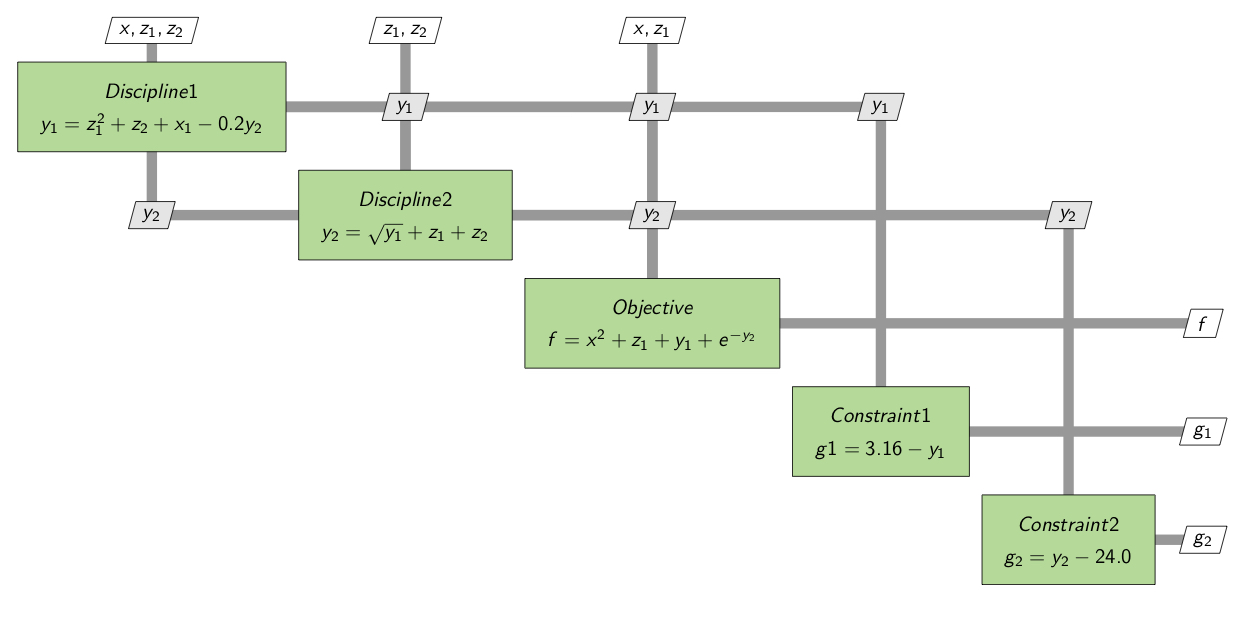
The following XDSM diagram shows the SellarMDA component equations and their inputs and outputs. Through the different recorders we can access the different parts of the model. We’ll take you through an example of each object and relate it back to the diagram.
Driver#
If we want to view the convergence of the model, the best place to find that by looking at the cases
recorded by the driver. By default, a recorder attached to a driver will record the design variables,
constraints and objectives, so we will print them for the model at the end of the optimization. We’ll
use the helper methods like get_objectives, get_design_vars, get_constraints to return the info
we’re seeking.
# Instantiate your CaseReader
cr = om.CaseReader(prob.get_outputs_dir() / "advanced_case_recording.sql")

# List driver cases (do not recurse to system/solver cases)
driver_cases = cr.list_cases('driver', recurse=False)
last_case = cr.get_case(driver_cases[-1])

objectives = last_case.get_objectives()
design_vars = last_case.get_design_vars()
constraints = last_case.get_constraints()

print(objectives['obj'])
print(design_vars['x'])
print(design_vars['z'])
print(constraints['con1'])
print(constraints['con2'])
| driver |
|---|
| rank0:ScipyOptimize_SLSQP|0 |
| rank0:ScipyOptimize_SLSQP|1 |
| rank0:ScipyOptimize_SLSQP|2 |
| rank0:ScipyOptimize_SLSQP|3 |
| rank0:ScipyOptimize_SLSQP|4 |
| rank0:ScipyOptimize_SLSQP|5 |
| rank0:ScipyOptimize_SLSQP|6 |
| rank0:ScipyOptimize_SLSQP|7 |
| rank0:ScipyOptimize_SLSQP|8 |
| rank0:ScipyOptimize_SLSQP|9 |
| rank0:ScipyOptimize_SLSQP|10 |
| rank0:ScipyOptimize_SLSQP|11 |
| rank0:ScipyOptimize_SLSQP|12 |
| rank0:ScipyOptimize_SLSQP|13 |
[3.18339395]
[1.79200776e-16]
[1.97763888e+00 7.74994687e-15]
[-1.65163438e-10]
[-20.24472223]
Plotting Design Variables#
When inspecting or debugging a model, it can be helpful to visualize the path of the design variables to their final values. To do this, we can list the cases of the driver and plot the data with respect to the iteration number.
import matplotlib.pyplot as plt

# Instantiate your CaseReader
cr = om.CaseReader(prob.get_outputs_dir() / "advanced_case_recording.sql")

# Get driver cases (do not recurse to system/solver cases)
driver_cases = cr.get_cases('driver', recurse=False)

# Plot the path the design variables took to convergence
# Note that there are two lines in the right plot because "Z"
# contains two variables that are being optimized
dv_x_values = []
dv_z_values = []
for case in driver_cases:
    dv_x_values.append(case['x'])
    dv_z_values.append(case['z'])

fig, (ax1, ax2) = plt.subplots(1, 2)
fig.subplots_adjust(left=None, bottom=None, right=None, top=None, wspace=0.5, hspace=None)

ax1.plot(np.arange(len(dv_x_values)), np.array(dv_x_values))
ax1.set(xlabel='Iterations', ylabel='Design Var: X', title='Optimization History')
ax1.grid()

ax2.plot(np.arange(len(dv_z_values)), np.array(dv_z_values))
ax2.set(xlabel='Iterations', ylabel='Design Var: Z', title='Optimization History')
ax2.grid()

plt.show()
<Figure size 640x480 with 2 Axes>
Problem#
A Problem recorder is best if you want to record an arbitrary case before or after a running the
model. In our case, we have placed our point at the end of the model.
# Instantiate your CaseReader
cr = om.CaseReader(prob.get_outputs_dir() / "advanced_case_recording.sql")

# get list of cases recorded on problem
problem_cases = cr.list_cases('problem')

# get list of variables recorded on problem
problem_vars = cr.list_source_vars('problem')
print(problem_vars['outputs'])

# get the recorded case and check values
case = cr.get_case('final_state')
print(case.get_design_vars())
print(case.get_constraints())
print(case.get_objectives())
| problem |
|---|
| final_state |
| inputs | outputs | residuals |
|---|---|---|
| x | ||
| z | ||
| con1 | ||
| con2 | ||
| y1 | ||
| y2 | ||
| obj |
['x', 'z', 'con1', 'con2', 'y1', 'y2', 'obj']
{'z': array([1.97763888e+00, 7.74994687e-15]), 'x': array([1.79200776e-16])}
{'con1': array([-1.65163438e-10]), 'con2': array([-20.24472223])}
{'obj': array([3.18339395])}
System#
Suppose we want to know the values of the inputs to the objective function.
For this we will use the system recorder. Using the list_cases method, we’ll get the list of
cases that were recorded by the objective component root.obj_comp. Then we use get_case to
get each case and determine the input names using the keys of the case’s inputs dictionary.
Since we want to find the values going into the objective function for each execution,
we iterate through those 14 cases and get the values in each.
# Instantiate your CaseReader
cr = om.CaseReader(prob.get_outputs_dir() / "advanced_case_recording.sql")

# Get a list of cases for the objective component
system_cases = cr.list_cases('root.obj_cmp', recurse=False)

# Number of cases recorded for 'obj_cmp'
print(f"Number of cases: {len(system_cases)}")

for case_num, case_id in enumerate(system_cases):
    case = cr.get_case(case_id)

    # Get the names of all the inputs to the objective component
    inputs = case.inputs.keys()

    # Get the rounded value of each input (as a python list)
    values = [(name, case[name].round(10).tolist()) for name in inputs]

    # Print the input values for this case
    print(f"{case_num:>2}: {values}")
| root.obj_cmp |
|---|
| rank0:ScipyOptimize_SLSQP|0|root._solve_nonlinear|0|NLRunOnce|0|obj_cmp._solve_nonlinear|0 |
| rank0:ScipyOptimize_SLSQP|1|root._solve_nonlinear|1|NLRunOnce|0|obj_cmp._solve_nonlinear|1 |
| rank0:ScipyOptimize_SLSQP|2|root._solve_nonlinear|2|NLRunOnce|0|obj_cmp._solve_nonlinear|2 |
| rank0:ScipyOptimize_SLSQP|3|root._solve_nonlinear|3|NLRunOnce|0|obj_cmp._solve_nonlinear|3 |
| rank0:ScipyOptimize_SLSQP|4|root._solve_nonlinear|4|NLRunOnce|0|obj_cmp._solve_nonlinear|4 |
| rank0:ScipyOptimize_SLSQP|5|root._solve_nonlinear|5|NLRunOnce|0|obj_cmp._solve_nonlinear|5 |
| rank0:ScipyOptimize_SLSQP|6|root._solve_nonlinear|6|NLRunOnce|0|obj_cmp._solve_nonlinear|6 |
| rank0:ScipyOptimize_SLSQP|7|root._solve_nonlinear|7|NLRunOnce|0|obj_cmp._solve_nonlinear|7 |
| rank0:ScipyOptimize_SLSQP|8|root._solve_nonlinear|8|NLRunOnce|0|obj_cmp._solve_nonlinear|8 |
| rank0:ScipyOptimize_SLSQP|9|root._solve_nonlinear|9|NLRunOnce|0|obj_cmp._solve_nonlinear|9 |
| rank0:ScipyOptimize_SLSQP|10|root._solve_nonlinear|10|NLRunOnce|0|obj_cmp._solve_nonlinear|10 |
| rank0:ScipyOptimize_SLSQP|11|root._solve_nonlinear|11|NLRunOnce|0|obj_cmp._solve_nonlinear|11 |
| rank0:ScipyOptimize_SLSQP|12|root._solve_nonlinear|12|NLRunOnce|0|obj_cmp._solve_nonlinear|12 |
| rank0:ScipyOptimize_SLSQP|13|root._solve_nonlinear|13|NLRunOnce|0|obj_cmp._solve_nonlinear|13 |
Number of cases: 14
 0: [('obj_cmp.x', [1.0]), ('obj_cmp.y1', [25.5883023699]), ('obj_cmp.y2', [12.0584881506]), ('obj_cmp.z', [5.0, 2.0])]
 1: [('obj_cmp.x', [1.0]), ('obj_cmp.y1', [25.5883023699]), ('obj_cmp.y2', [12.0584881506]), ('obj_cmp.z', [5.0, 2.0])]
 2: [('obj_cmp.x', [0.0]), ('obj_cmp.y1', [8.3303475222]), ('obj_cmp.y2', [6.6613736358]), ('obj_cmp.z', [2.977394348, 0.7977451458])]
 3: [('obj_cmp.x', [0.0]), ('obj_cmp.y1', [4.1743070349]), ('obj_cmp.y2', [4.2862241911]), ('obj_cmp.z', [2.2431120955, 0.0])]
 4: [('obj_cmp.x', [0.0014523042]), ('obj_cmp.y1', [3.3018190875]), ('obj_cmp.y2', [3.8338028461]), ('obj_cmp.z', [2.0167120153, 0.0])]
 5: [('obj_cmp.x', [0.0]), ('obj_cmp.y1', [3.1752069972]), ('obj_cmp.y2', [3.763822104]), ('obj_cmp.z', [1.981911052, 0.0])]
 6: [('obj_cmp.x', [0.0]), ('obj_cmp.y1', [3.1615493902]), ('obj_cmp.y2', [3.7561492602]), ('obj_cmp.z', [1.9780746301, 0.0])]
 7: [('obj_cmp.x', [0.0]), ('obj_cmp.y1', [3.1601567921]), ('obj_cmp.y2', [3.7553659683]), ('obj_cmp.z', [1.9776829841, 0.0])]
 8: [('obj_cmp.x', [0.0]), ('obj_cmp.y1', [3.1600158611]), ('obj_cmp.y2', [3.7552866895]), ('obj_cmp.z', [1.9776433447, 0.0])]
 9: [('obj_cmp.x', [0.0]), ('obj_cmp.y1', [3.1600016041]), ('obj_cmp.y2', [3.7552786693]), ('obj_cmp.z', [1.9776393346, 0.0])]
10: [('obj_cmp.x', [0.0]), ('obj_cmp.y1', [3.1600001606]), ('obj_cmp.y2', [3.7552778573]), ('obj_cmp.z', [1.9776389286, 1e-10])]
11: [('obj_cmp.x', [0.0]), ('obj_cmp.y1', [3.1600000163]), ('obj_cmp.y2', [3.7552777761]), ('obj_cmp.z', [1.977638888, 0.0])]
12: [('obj_cmp.x', [0.0]), ('obj_cmp.y1', [3.1600000016]), ('obj_cmp.y2', [3.7552777678]), ('obj_cmp.z', [1.9776388839, 0.0])]
13: [('obj_cmp.x', [0.0]), ('obj_cmp.y1', [3.1600000002]), ('obj_cmp.y2', [3.755277767]), ('obj_cmp.z', [1.9776388835, 0.0])]
Solver#
Similar to the system recorder, we can query the cases recorded by the solver. You can also
access the values of inputs to the equation with the solver but in this case we’ll focus on the
coupling variables y1 and y2.
We’ll use list_cases to get the cases recorded for 'root.cycle.nonlinear_solver', find out how many
cases there are and plot a subset of the solver iterations (covering multiple driver iterations)
to see the final convergence.
# Instantiate your CaseReader
cr = om.CaseReader(prob.get_outputs_dir() / "advanced_case_recording.sql")

# Get list of cases, without displaying them
solver_cases = cr.list_cases('root.cycle.nonlinear_solver', out_stream=None)

# we will plot the last half of the iterations
num_cases = len(solver_cases)
sub_cases = num_cases//2
iterations = np.arange(num_cases-sub_cases, num_cases)

# Plot the final convergence of the two coupling variables
y1_history = []
y2_history = []

for case_id in solver_cases[-sub_cases:]:
    case = cr.get_case(case_id)
    y1_history.append(case['y1'])
    y2_history.append(case['y2'])

fig, (ax1, ax2) = plt.subplots(2, 1)

ax1.plot(iterations, np.array(y1_history))
ax1.set(ylabel='Coupling Output: y1', title='Solver History')
ax1.grid()

ax2.plot(iterations, np.array(y2_history))
ax2.set(ylabel='Coupling Parameter: y2', xlabel='Iterations')
ax2.grid()

plt.show()

# Get the final values
print(f"Number of cases: {len(solver_cases)}")
print("Final values:")
case = cr.get_case(solver_cases[-1])
print('  y1:', case['y1'])
print('  y2:', case['y2'])
<Figure size 640x480 with 2 Axes>
Number of cases: 76
Final values:
  y1: [3.16]
  y2: [3.75527777]