Hohmann Transfer Example - Optimizing a Spacecraft Manuever#
This example will demonstrate the use of OpenMDAO for optimizing a simple orbital mechanics problem. We seek the minimum possible delta-V to transfer a spacecraft from Low Earth Orbit (LEO) to geostationary orbit (GEO) using a two-impulse Hohmann Transfer.
The Hohmann Transfer is a maneuver which minimizes the delta-V for transferring a spacecraft from one circular orbit to another. Hohmann transfers have a practical application in that they can be used to transfer satellites from LEO parking orbits to geostationary orbit.
To do so, the vehicle first imparts a delta-V along the velocity vector while in LEO. This boosts apogee radius to the radius of the geostationary orbit (42164 km). In this model we will model this delta-V as an impulsive maneuver which changes the spacecraft’s velocity instantaneously.
We will assume that the first impulse is performed at the ascending node in LEO. Thus perigee of the transfer orbit is coincident with the ascending node of the transfer orbit. Apogee of the transfer orbit is thus coincident with the descending node, where we will perform the second impulse.
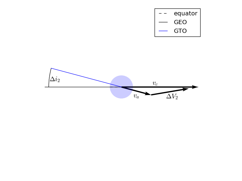
After the first impulse, the spacecraft coasts to apogee. Once there it performs a second impulsive burn along the velocity vector to raise perigee radius to the radius of GEO, thus circularizing the orbit.
Simple, right? The issue is that, unless they launch from the equator, launch vehicles do not put satellites in a low Earth parking orbit with the same inclination as geostationary orbit. For instance, a due-east launch from Kennedy Space Center will result in a parking orbit with an inclination of 28.5 degrees. We therefore need to change the inclination of our satellite during its two impulsive burn maneuvers. The question is, what change in inclination at each burn will result in the minimum possible delta-V?
The trajectory optimization problem can thus be stated as:
The total \({\Delta} V\) is the sum of the two impulsive \({\Delta Vs}\).
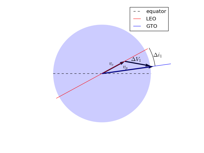
The component of the \({\Delta V}\) in the orbital plane is along the local horizontal plane. The orbit-normal component is in the direction of the desired inclination change. Knowing the velocity magnitude before (\({v_c}\)) and after (\({v_p}\)) the impulse, and the change in inclination due to the impulse (\({\Delta i}\)), the \({\Delta V}\) is then computed from the law of cosines:
In the first impulse, \({v_1}\) is the circular velocity in LEO. In this case \({v_c}\) refers to the circular velocity in geostationary orbit, and \({v_a}\) is the velocity at apogee of the transfer orbit.
We can compute the circular velocity in either orbit from the following equation:
where \({\mu}\) is the gravitational parameter of the Earth and \({r}\) is the distance from the center of the Earth.
The velocity after the first impulse is the periapsis velocity of the transfer orbit. This can be solved for based on what we know about the orbit.
The specific angular momentum of the transfer orbit is constant. At periapsis, it is simply the product of the velocity and radius. Therefore, rearranging we have:
The specific angular momentum can also be computed as:
Where \({p}\) is the semilatus rectum of the orbit and \({\mu}\) is the gravitational parameter of the central body.
The semilatus rectum is computed as:
Where \({a}\) and \({e}\) are the semi-major axis and eccentricity of the transfer orbit, respectively. Since we know \({r_a}\) and \({r_p}\) of the transfer orbit, it’s semimajor axis is simply:
The eccentricity is known by the relationship of \({a}\) and \({e}\) to \({r_p}\) (or \({r_a}\)):
Thus we can compute periapsis velocity based on the periapsis and apoapsis radii of the transfer orbit, and the gravitational parameter of the central body.
For the second impulse, the final velocity is the circular velocity of the final orbit, which can be computed in the same way as the circular velocity of the initial orbit. The initial velocity at the second impulse is the apoapsis velocity of the transfer orbit, which is:
Having already computed the specific angular momentum of the transfer orbit, this is easily computed.
Finally we have the necessary calculations to compute the \({\Delta V}\) of the Hohmann transfer with a plane change.
Components#
The first component we define computes the circular velocity given the radius from the center of the central body and the gravitational parameter of the central body.
import numpy as np
import openmdao.api as om


class VCircComp(om.ExplicitComponent):
    """
    Computes the circular orbit velocity given a radius and gravitational
    parameter.
    """
    def initialize(self):
        pass

    def setup(self):
        self.add_input('r',
                       val=1.0,
                       desc='Radius from central body',
                       units='km')

        self.add_input('mu',
                       val=1.0,
                       desc='Gravitational parameter of central body',
                       units='km**3/s**2')

        self.add_output('vcirc',
                        val=1.0,
                        desc='Circular orbit velocity at given radius '
                             'and gravitational parameter',
                        units='km/s')

        self.declare_partials(of='vcirc', wrt='r')
        self.declare_partials(of='vcirc', wrt='mu')

    def compute(self, inputs, outputs):
        r = inputs['r']
        mu = inputs['mu']

        outputs['vcirc'] = np.sqrt(mu / r)

    def compute_partials(self, inputs, partials):
        r = inputs['r']
        mu = inputs['mu']
        vcirc = np.sqrt(mu / r)

        partials['vcirc', 'mu'] = 0.5 / (r * vcirc)
        partials['vcirc', 'r'] = -0.5 * mu / (vcirc * r ** 2)
The transfer orbit component computes the velocity magnitude at periapsis and apoapsis of an orbit, given the radii of periapsis and apoapsis, and the gravitational parameter of the central body.
class TransferOrbitComp(om.ExplicitComponent):
    def initialize(self):
        pass

    def setup(self):
        self.add_input('mu',
                       val=398600.4418,
                       desc='Gravitational parameter of central body',
                       units='km**3/s**2')
        self.add_input('rp', val=7000.0, desc='periapsis radius', units='km')
        self.add_input('ra', val=42164.0, desc='apoapsis radius', units='km')

        self.add_output('vp', val=0.0, desc='periapsis velocity', units='km/s')
        self.add_output('va', val=0.0, desc='apoapsis velocity', units='km/s')

        # We're going to be lazy and ask OpenMDAO to approximate our
        # partials with finite differencing here.
        self.declare_partials(of='*', wrt='*', method='fd')

    def compute(self, inputs, outputs):
        mu = inputs['mu']
        rp = inputs['rp']
        ra = inputs['ra']

        a = (ra + rp) / 2.0
        e = (a - rp) / a
        p = a * (1.0 - e ** 2)
        h = np.sqrt(mu * p)

        outputs['vp'] = h / rp
        outputs['va'] = h / ra
The delta-V component is used to compute the delta-V performed in changing the velocity vector, giving the magnitudes of the initial and final velocities and the angle between them.
class DeltaVComp(om.ExplicitComponent):
    """
    Compute the delta-V performed given the magnitude of two velocities
    and the angle between them.
    """
    def initialize(self):
        pass

    def setup(self):
        self.add_input('v1', val=1.0, desc='Initial velocity', units='km/s')
        self.add_input('v2', val=1.0, desc='Final velocity', units='km/s')
        self.add_input('dinc', val=1.0, desc='Plane change', units='rad')

        # Note:  We're going to use trigonometric functions on dinc.  The
        # automatic unit conversion in OpenMDAO comes in handy here.

        self.add_output('delta_v', val=0.0, desc='Delta-V', units='km/s')

        self.declare_partials(of='delta_v', wrt='v1')
        self.declare_partials(of='delta_v', wrt='v2')
        self.declare_partials(of='delta_v', wrt='dinc')

    def compute(self, inputs, outputs):
        v1 = inputs['v1']
        v2 = inputs['v2']
        dinc = inputs['dinc']

        outputs['delta_v'] = np.sqrt(v1 ** 2 + v2 ** 2 - 2.0 * v1 * v2 * np.cos(dinc))

    def compute_partials(self, inputs, partials):
        v1 = inputs['v1']
        v2 = inputs['v2']
        dinc = inputs['dinc']

        delta_v = np.sqrt(v1 ** 2 + v2 ** 2 - 2.0 * v1 * v2 * np.cos(dinc))

        partials['delta_v', 'v1'] = 0.5 / delta_v * (2 * v1 - 2 * v2 * np.cos(dinc))
        partials['delta_v', 'v2'] = 0.5 / delta_v * (2 * v2 - 2 * v1 * np.cos(dinc))
        partials['delta_v', 'dinc'] = 0.5 / delta_v * (2 * v1 * v2 * np.sin(dinc))
Putting it all together#
Now we assemble the model for our problem.
Two instances of VCircComp are used to compute the velocity of the spacecraft in the initial and final circular orbits.
The TransferOrbitComp is used to compute the periapsis and apoapsis velocity of the spacecraft in the transfer orbit.
Now we can use the DeltaVComp to provide the magnitude of the delta-V at each of the two impulses.
We use two ExecComps to provide some simple calculations. One sums the delta-Vs of the two impulses to provide the total delta-V of the transfer. We will use this as the objective for the optimization.
The other ExecComp sums up the inclination change at each impulse. We will provide this to the driver as a constraint to ensure that our total inclination change meets our requirements.
Lastly, we provide unambiguous values and units for the gravitational parameter, the radii of the two circular orbits, and the delta-V to be performed at each of the two impulses.
We will use the initial and final radii of the orbits, and the inclination change at each of the two impulses as our design variables.
To run the model, we provide values for the design variables and invoke run_model.
To find the optimal solution for the model, we invoke run_driver, where we have
defined the driver of the problem to be ScipyOptimizeDriver.
prob = om.Problem()

model = prob.model

model.add_subsystem('leo', subsys=VCircComp(), promotes_inputs=[('r', 'r1'), 'mu'])
model.add_subsystem('geo', subsys=VCircComp(), promotes_inputs=[('r', 'r2'), 'mu'])

model.add_subsystem('transfer', subsys=TransferOrbitComp(),
                    promotes_inputs=[('rp', 'r1'), ('ra', 'r2'), 'mu'])

model.add_subsystem('dv1', subsys=DeltaVComp(), promotes_inputs=[('dinc', 'dinc1')])

model.connect('leo.vcirc', 'dv1.v1')
model.connect('transfer.vp', 'dv1.v2')

model.add_subsystem('dv2', subsys=DeltaVComp(), promotes_inputs=[('dinc', 'dinc2')])

model.connect('transfer.va', 'dv2.v1')
model.connect('geo.vcirc', 'dv2.v2')

model.add_subsystem('dv_total',
                    subsys=om.ExecComp('delta_v=dv1+dv2',
                                       delta_v={'units': 'km/s'},
                                       dv1={'units': 'km/s'},
                                       dv2={'units': 'km/s'}),
                    promotes=['delta_v'])

model.connect('dv1.delta_v', 'dv_total.dv1')
model.connect('dv2.delta_v', 'dv_total.dv2')

model.add_subsystem('dinc_total',
                    subsys=om.ExecComp('dinc=dinc1+dinc2',
                                       dinc={'units': 'deg'},
                                       dinc1={'units': 'deg'},
                                       dinc2={'units': 'deg'}),
                    promotes=['dinc', 'dinc1', 'dinc2'])

prob.driver = om.ScipyOptimizeDriver()

model.add_design_var('dinc1', lower=0, upper=28.5)
model.add_design_var('dinc2', lower=0, upper=28.5)
model.add_constraint('dinc', lower=28.5, upper=28.5, scaler=1.0)
model.add_objective('delta_v', scaler=1.0)

# set defaults for our promoted variables to remove ambiguities in value and/or units
model.set_input_defaults('r1', val=6778.0)
model.set_input_defaults('r2', val=42164.0)
model.set_input_defaults('mu', val=398600.4418)
model.set_input_defaults('dinc1', val=0., units='deg')
model.set_input_defaults('dinc2', val=28.5, units='deg')

# Setup the problem
prob.setup()

# Execute the model with the given inputs
prob.run_model()

print('Delta-V (km/s):', prob['delta_v'][0])
Delta-V (km/s): 4.221581425832456
print('Inclination change split (deg):', prob['dinc1'][0], prob['dinc2'][0])
Inclination change split (deg): 0.0 28.5
prob.run_driver()
Optimization terminated successfully    (Exit mode 0)
            Current function value: 4.196344171917739
            Iterations: 6
            Function evaluations: 6
            Gradient evaluations: 6
Optimization Complete
-----------------------------------
Problem: problem
Driver:  ScipyOptimizeDriver
  success     : True
  iterations  : 7
  runtime     : 6.4084E-02 s
  model_evals : 7
  model_time  : 1.5081E-03 s
  deriv_evals : 6
  deriv_time  : 4.8446E-02 s
  exit_status : SUCCESS
print('Optimized Delta-V (km/s):', prob['delta_v'][0])
Optimized Delta-V (km/s): 4.196344171917739
print('Inclination change split (deg):', prob['dinc1'][0], prob['dinc2'][0])
Inclination change split (deg): 2.22213125891072 26.277868741089282
Summary#
We built a model representing a Hohmann transfer with a plane change. This model utilized components with both analytic partial derivatives and approximated partials using finite differencing. We utilized ExecComps for some simple calculations to reduce the amount of code we needed to write. Finally, we used this model to demonstrate that performing the necessary plane change entirely at apoapsis is somewhat less optimal, from a delta-V standpoint, than performing some of the plane change at the first impulse.