Sellar - A Two-Discipline Problem with a Nonlinear Solver#
In the monodisciplinary tutorials, we built and optimized models comprised of only a single component. Now, we’ll work through a slightly more complex problem that involves two disciplines, and hence two main components. You’ll learn how to group components together into a larger model and how to use a NonlinearBlockGaussSeidel nonlinear solver to converge a group with coupled components.
The Sellar problem is a two-discipline toy problem with each discipline described by a single equation.
There isn’t any physical significance to the equations, it’s just a compact example to use as a means of understanding
simple coupled models.
The output of each component feeds into the input of the other, which creates a coupled model that needs to
be converged in order for the outputs to be valid.
You can see the coupling between the two disciplines show up through the \(y_1\) and \(y_2\) variables in the following diagram that describes the problem structure: 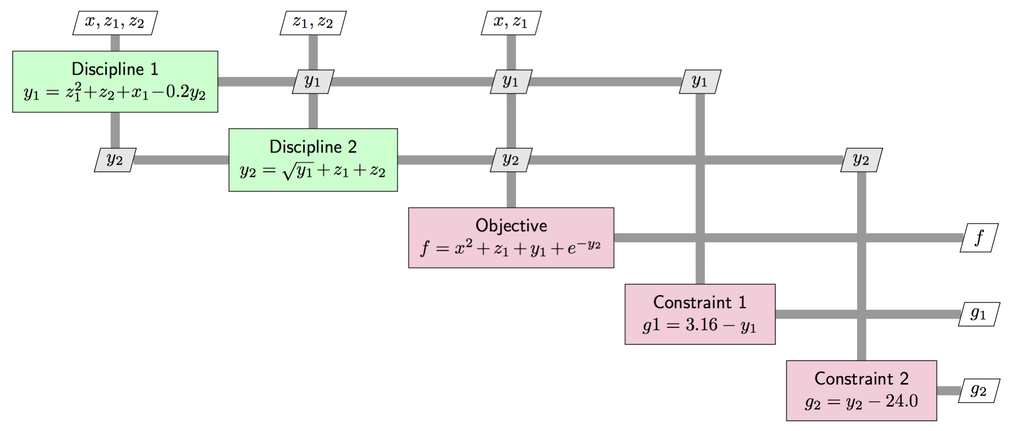
Building the Disciplinary Components#
In the following component definitions, there is a call to declare_partials in the setup_partials method that looks like this:
self.declare_partials('*', '*', method='fd')
This command tells OpenMDAO to approximate all the partial derivatives of that component using finite difference. The default settings will use forward difference with an absolute step size of 1e-6, but you can change the FD settings to work well for your component.
import numpy as np
import openmdao.api as om


class SellarDis1(om.ExplicitComponent):
    """
    Component containing Discipline 1 -- no derivatives version.
    """

    def setup(self):

        # Global Design Variable
        self.add_input('z', val=np.zeros(2))

        # Local Design Variable
        self.add_input('x', val=0.)

        # Coupling parameter
        self.add_input('y2', val=1.0)

        # Coupling output
        self.add_output('y1', val=1.0)

    def setup_partials(self):
        # Finite difference all partials.
        self.declare_partials('*', '*', method='fd')

    def compute(self, inputs, outputs):
        """
        Evaluates the equation
        y1 = z1**2 + z2 + x1 - 0.2*y2
        """
        z1 = inputs['z'][0]
        z2 = inputs['z'][1]
        x1 = inputs['x']
        y2 = inputs['y2']

        outputs['y1'] = z1**2 + z2 + x1 - 0.2*y2
class SellarDis2(om.ExplicitComponent):
    """
    Component containing Discipline 2 -- no derivatives version.
    """

    def setup(self):
        # Global Design Variable
        self.add_input('z', val=np.zeros(2))

        # Coupling parameter
        self.add_input('y1', val=1.0)

        # Coupling output
        self.add_output('y2', val=1.0)

    def setup_partials(self):
        # Finite difference all partials.
        self.declare_partials('*', '*', method='fd')

    def compute(self, inputs, outputs):
        """
        Evaluates the equation
        y2 = y1**(.5) + z1 + z2
        """

        z1 = inputs['z'][0]
        z2 = inputs['z'][1]
        y1 = inputs['y1']

        # Note: this may cause some issues. However, y1 is constrained to be
        # above 3.16, so lets just let it converge, and the optimizer will
        # throw it out
        if y1.real < 0.0:
            y1 *= -1

        outputs['y2'] = y1**.5 + z1 + z2
Grouping and Connecting Components#
We now want to build in OpenMDAO the model that is represented by the XDSM diagram above. We’ve defined the two disciplinary components, but there are still the three outputs of the model that need to be computed. Additionally, since we have the computations split up into multiple components, we need to group them all together and tell OpenMDAO how to pass data between them.
class SellarMDA(om.Group):
    """
    Group containing the Sellar MDA.
    """

    def setup(self):
        cycle = self.add_subsystem('cycle', om.Group(), promotes=['*'])
        cycle.add_subsystem('d1', SellarDis1(), promotes_inputs=['x', 'z', 'y2'],
                            promotes_outputs=['y1'])
        cycle.add_subsystem('d2', SellarDis2(), promotes_inputs=['z', 'y1'],
                            promotes_outputs=['y2'])

        self.set_input_defaults('x', 1.0)
        self.set_input_defaults('z', np.array([5.0, 2.0]))

        # Nonlinear Block Gauss Seidel is a gradient free solver
        cycle.nonlinear_solver = om.NonlinearBlockGS()

        self.add_subsystem('obj_cmp', om.ExecComp('obj = x**2 + z[1] + y1 + exp(-y2)',
                                                  z=np.array([0.0, 0.0]), x=0.0),
                           promotes=['x', 'z', 'y1', 'y2', 'obj'])

        self.add_subsystem('con_cmp1', om.ExecComp('con1 = 3.16 - y1'), promotes=['con1', 'y1'])
        self.add_subsystem('con_cmp2', om.ExecComp('con2 = y2 - 24.0'), promotes=['con2', 'y2'])
We’re working with a new class: Group. This is the container that lets you build up complex model hierarchies. Groups can contain other groups, components, or combinations of groups and components.
You can directly create instances of Group to work with, or you can subclass from it to define your own custom
groups. We’re doing both of these things above. First, we defined our own custom Group subclass called SellarMDA.
In our run script, we created an instance of SellarMDA to actually run it.
Then, inside the setup method of SellarMDA we’re also working directly with a Group instance by adding the subsystem cycle:
prob = om.Problem()
cycle = prob.model.add_subsystem('cycle', om.Group(), promotes=['*'])
cycle.add_subsystem('d1', SellarDis1(), promotes_inputs=['x', 'z', 'y2'], promotes_outputs=['y1'])
cycle.add_subsystem('d2', SellarDis2(), promotes_inputs=['z', 'y1'], promotes_outputs=['y2'])

# Nonlinear Block Gauss-Seidel is a gradient-free solver
cycle.nonlinear_solver = om.NonlinearBlockGS()
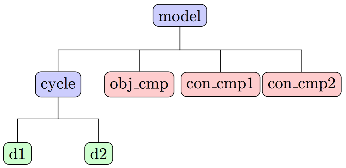
Our SellarMDA Group, when instantiated, will have a three-level hierarchy, with itself as the topmost level, as
illustrated in the following figure:
Why do we create the cycle subgroup?#
There is a circular data dependency between d1 and d2 that needs to be converged with a nonlinear solver in order to get a valid answer. It’s a bit more efficient to put these two components into their own subgroup, so that we can iteratively converge them by themselves, before moving on to the rest of the calculations in the model. Models with cycles in them are often referred to as “Multidisciplinary Analyses” or MDA for short. You can pick which kind of solver you would like to use to converge the MDA. The most common choices are:
The NonlinearBlockGaussSeidel solver, also sometimes called a “fixed-point iteration solver,” is a gradient-free method
that works well in many situations.
More tightly-coupled problems, or problems with instances of ImplicitComponent that don’t implement their own solve_nonlinear method, will require the Newton solver.
Note
OpenMDAO comes with other nonlinear solvers you can use if they suit your problem. Here is the complete list of OpenMDAO’s nonlinear solvers.
The subgroup, named cycle, is useful here, because it contains the multidisciplinary coupling of the Sellar problem.
This allows us to assign the nonlinear solver to cycle to just converge those two components, before moving on to the final
calculations for the obj_cmp, con_cmp1, and con_cmp2 to compute the actual outputs of the problem.
Promoting variables with the same name connects them#
The data connections in this model are made via promotion. OpenMDAO will look at each level of the hierarchy and connect all output-input pairs that have the same names. When an input is promoted on multiple components, you can use “set_input_defaults” to define the common initial value.
ExecComp is a helper component for quickly defining components for simple equations#
A lot of times in your models, you need to define a new variable as a simple function of other variables.
OpenMDAO provides a helper component to make this easier, called ExecComp.
It’s fairly flexible, allowing you to work with scalars or arrays, to work with units, and to call basic math
functions (e.g. sin or exp). We have used ExecComp in this model to calculate our
objectives and constraints.