Simple Optimization using Simultaneous Derivatives

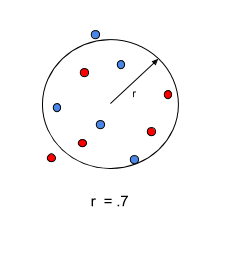
Simple Optimization using Simultaneous Derivatives#

Consider a set of points in 2-d space that are to be arranged along a circle such that the radius of the circle is maximized, subject to constraints. We start out with the points randomly distributed within a unit circle centered about the origin. The locations of our points are determined by the values of the x and y arrays defined in our problem.

import numpy as np
import openmdao.api as om

SIZE = 10

p = om.Problem()

p.model.add_subsystem('arctan_yox', om.ExecComp('g=arctan(y/x)', has_diag_partials=True,
                                                g=np.ones(SIZE), x=np.ones(SIZE), y=np.ones(SIZE)),
                      promotes_inputs=['x', 'y'])

p.model.add_subsystem('circle', om.ExecComp('area=pi*r**2'), promotes_inputs=['r'])

p.model.add_subsystem('r_con', om.ExecComp('g=x**2 + y**2 - r', has_diag_partials=True,
                                           g=np.ones(SIZE), x=np.ones(SIZE), y=np.ones(SIZE)),
                      promotes_inputs=['r', 'x', 'y'])

thetas = np.linspace(0, np.pi/4, SIZE)
p.model.add_subsystem('theta_con', om.ExecComp('g = x - theta', has_diag_partials=True,
                                               g=np.ones(SIZE), x=np.ones(SIZE),
                                               theta=thetas))
p.model.add_subsystem('delta_theta_con', om.ExecComp('g = even - odd', has_diag_partials=True,
                                                     g=np.ones(SIZE//2), even=np.ones(SIZE//2),
                                                     odd=np.ones(SIZE//2)))

p.model.add_subsystem('l_conx', om.ExecComp('g=x-1', has_diag_partials=True, g=np.ones(SIZE), x=np.ones(SIZE)),
                      promotes_inputs=['x'])

IND = np.arange(SIZE, dtype=int)
ODD_IND = IND[1::2]  # all odd indices
EVEN_IND = IND[0::2]  # all even indices

p.model.connect('arctan_yox.g', 'theta_con.x')
p.model.connect('arctan_yox.g', 'delta_theta_con.even', src_indices=EVEN_IND)
p.model.connect('arctan_yox.g', 'delta_theta_con.odd', src_indices=ODD_IND)

p.driver = om.ScipyOptimizeDriver()
p.driver.options['optimizer'] = 'SLSQP'
p.driver.options['disp'] = False

# set up dynamic total coloring here
p.driver.declare_coloring()

p.model.add_design_var('x')
p.model.add_design_var('y')
p.model.add_design_var('r', lower=.5, upper=10)

# nonlinear constraints
p.model.add_constraint('r_con.g', equals=0)

p.model.add_constraint('theta_con.g', lower=-1e-5, upper=1e-5, indices=EVEN_IND)
p.model.add_constraint('delta_theta_con.g', lower=-1e-5, upper=1e-5)

# this constrains x[0] to be 1 (see definition of l_conx)
p.model.add_constraint('l_conx.g', equals=0, linear=False, indices=[0,])

# linear constraint
p.model.add_constraint('y', equals=0, indices=[0,], linear=True)

p.model.add_objective('circle.area', ref=-1)

p.setup(mode='fwd')

# the following were randomly generated using np.random.random(10)*2-1 to randomly
# disperse them within a unit circle centered at the origin.
p.set_val('x', np.array([ 0.55994437, -0.95923447,  0.21798656, -0.02158783,  0.62183717,
                          0.04007379,  0.46044942, -0.10129622,  0.27720413, -0.37107886]))
p.set_val('y', np.array([ 0.52577864,  0.30894559,  0.8420792 ,  0.35039912, -0.67290778,
                         -0.86236787, -0.97500023,  0.47739414,  0.51174103,  0.10052582]))
p.set_val('r', .7)

p.run_driver()

print(p['circle.area'])

Full total jacobian for problem 'problem' was computed 3 times, taking 0.015835315999993327 seconds.
Total jacobian shape: (22, 21) 


Jacobian shape: (22, 21)  (13.42% nonzero)
FWD solves: 5   REV solves: 0
Total colors vs. total size: 5 vs 21  (76.19% improvement)

Sparsity computed using tolerance: 1e-25
Time to compute sparsity:   0.0158 sec
Time to compute coloring:   0.0027 sec
Memory to compute coloring:   0.6250 MB
Coloring created on: 2024-04-26 19:32:48

[3.14159265]

Total derivatives with respect to x and y will be solved for simultaneously based on the color of the points shown below. Note that we have two colors and our x and y design variables are of size 10. We have a third design variable, r, that is size 1. This means that if we don’t solve for derivatives simultaneously, we must perform 21 linear solves (10 + 10 + 1) to solve for total derivatives with respect to all of our design variables. But, since all of our design variables have only 5 colors, we can solve for all of our total derivatives using only 5 linear solves. This means that using simultaneous derivatives saves us 16 linear solves each time we compute our total derivatives.

Here’s our problem at the start of the optimization:

pre optimization

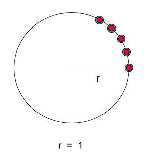
After the optimization, all of our points lie along the unit circle. The final radius is 1.0 (which corresponds to an area of PI) because we constrained our x[0] value to be 1.0.

pre optimization