Solving for Derivatives of Multiple Separable Constraints Using a Single Linear Solve

A set of constraints are separable when there are subsets of the design variables that don’t affect any of the responses. In other words, there is some subset of columns of the total-derivative Jacobian where none of those columns have nonzero values in any of the same rows. This kind of sparsity structure in the total-derivative Jacobian allows OpenMDAO to solve for multiple total derivatives simultaneously, which can dramatically reduce the cost of computing total derivatives. Remember that OpenMDAO solves the unified derivative equations to compute total derivatives.

\[ \begin{align*} \left[\frac{\partial \mathcal{R}}{\partial U}\right] \left[\frac{du}{dr}\right] = \left[ I \right] = \left[\frac{\partial \mathcal{R}}{\partial U}\right]^T \left[\frac{du}{dr}\right]^T . \end{align*} \]

When separable constraints are present, multiple right hand sides from \(\left[ I \right]\) can be combined into a single right-hand-side vector, and then total derivatives for multiple variables can be computed with a single linear solve. Normally, summing multiple right-hand-side vectors would result in the solution vector holding linear combinations of multiple derivatives:

\[\begin{split} \begin{gather} \frac{du_0}{dr_0} + \frac{du_0}{dr_2} + \cdots + \frac{du_0}{dr_n}\\ \vdots \\ \frac{du_m}{dr_0} + \frac{du_m}{dr_2} + \cdots + \frac{du_m}{dr_n}\\ \end{gather} \end{split}\]

However, because the problem is separable, we know that \(\frac{dy_i}{dx_j}=0\) for all \(i \ne j\) for seperable variables. Therefore, it is safe to do all the linear solves at the same time, and we can get a significant computational savings with no additional complexity of memory costs.

A Simple Example

Consider a notional optimization problem with 5 design variables (\(a, b, c, d, e\)), one objective (\(f\)), and three constraints (\(g_c, g_d, g_e\)). Normally with 5 design variables and 4 responses — 3 constraints + 1 objective — you would choose to use reverse mode since that would yield fewer linear solves. However, if the problem had the following partial derivative Jacobian structure, then it would be separable in forward mode, and we’ll show that because of that, forward mode is the preferred method.

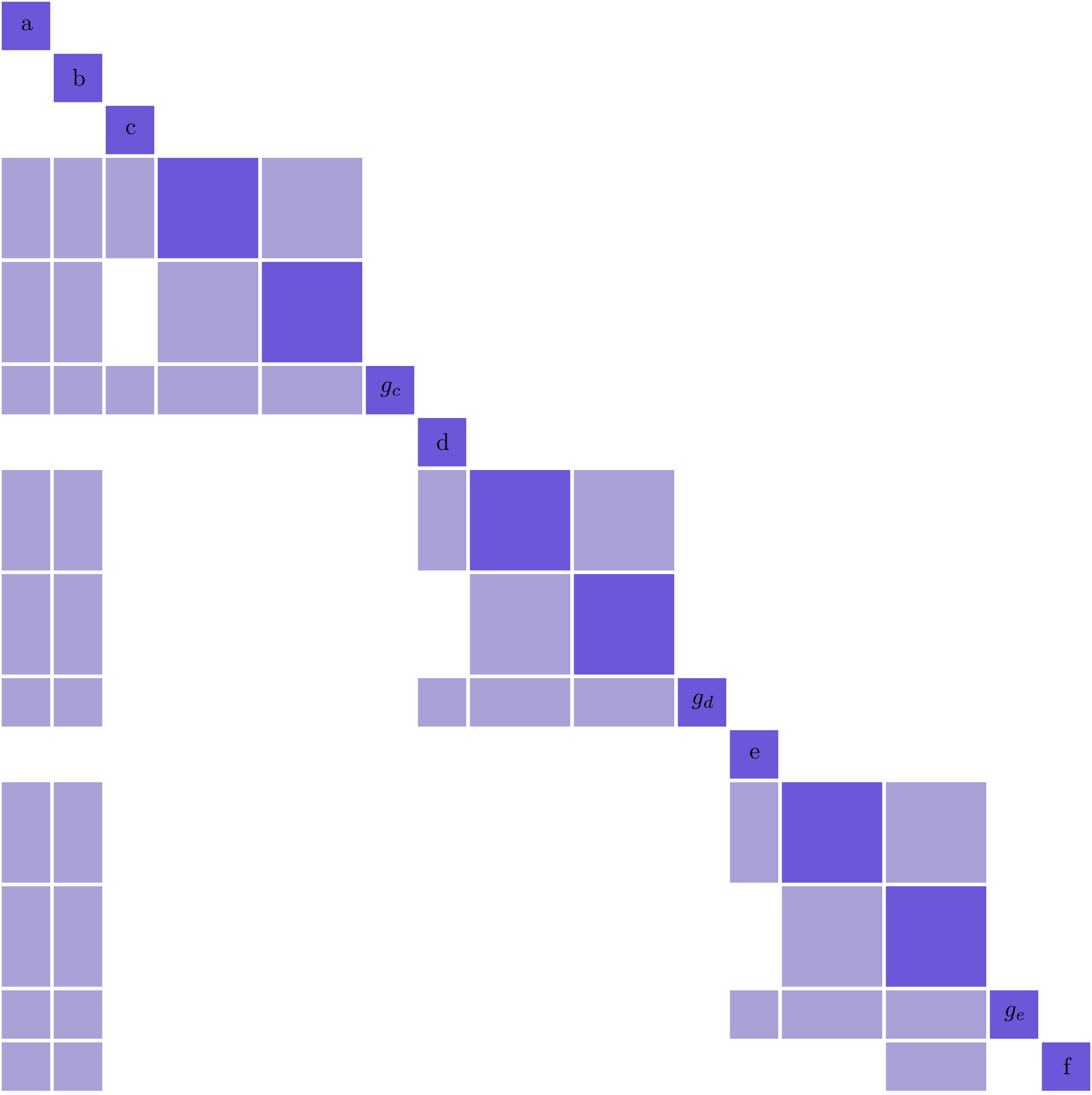
The two dense columns corresponding to \(a, b\) mean that all of the outputs depend on these variables and they must each get their own linear solves in forward mode.

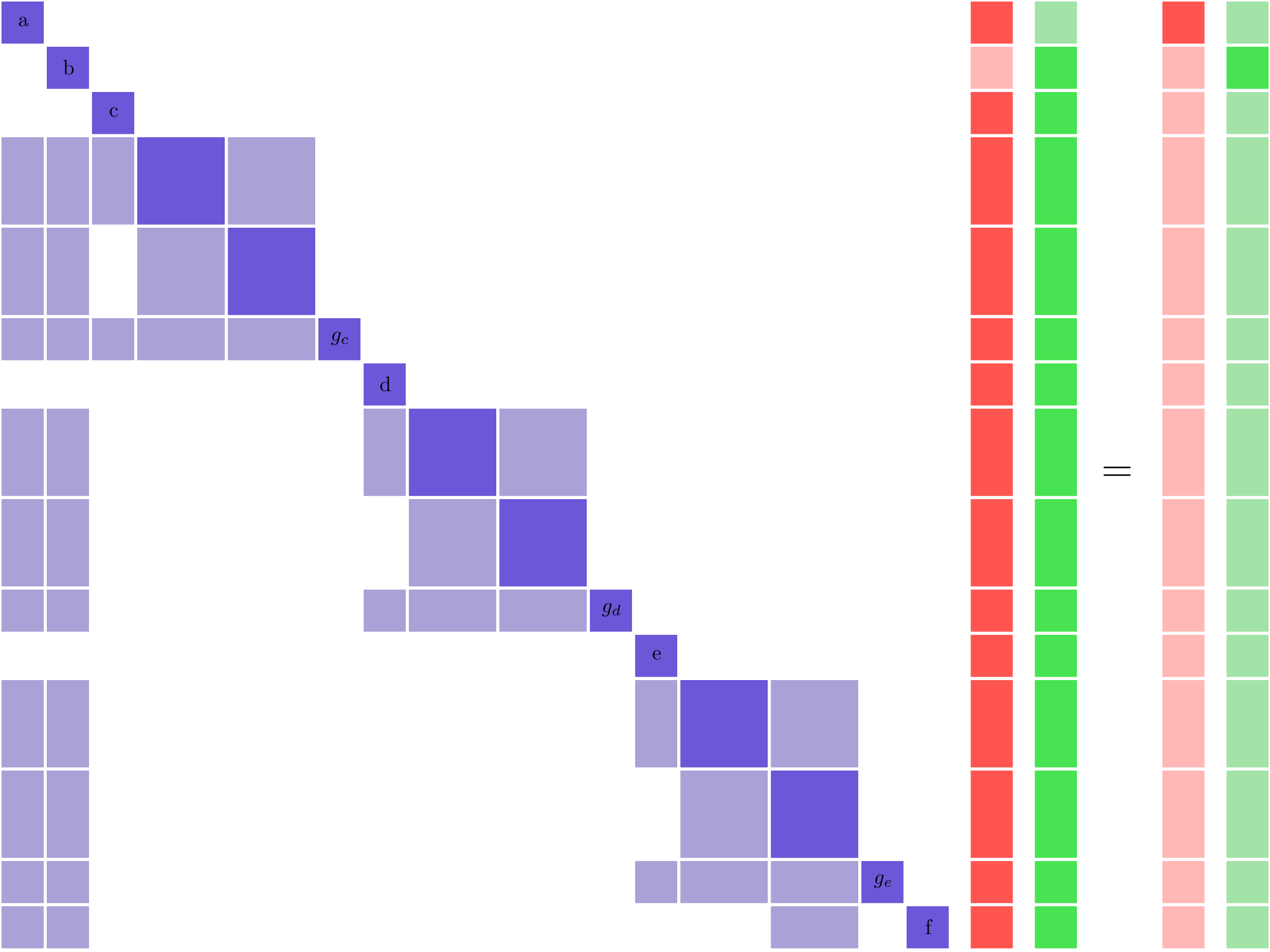
Normally, each of the remaining variables, (\(c, d, e\)), would also need their own linear solves, as shown below. In the solution and right-hand-side vectors, the zero values are denoted by the lighter-colored blocks. The nonzero values are denoted by the darker-colored blocks. Notice how the three solution vectors have no overlapping nonzero values.

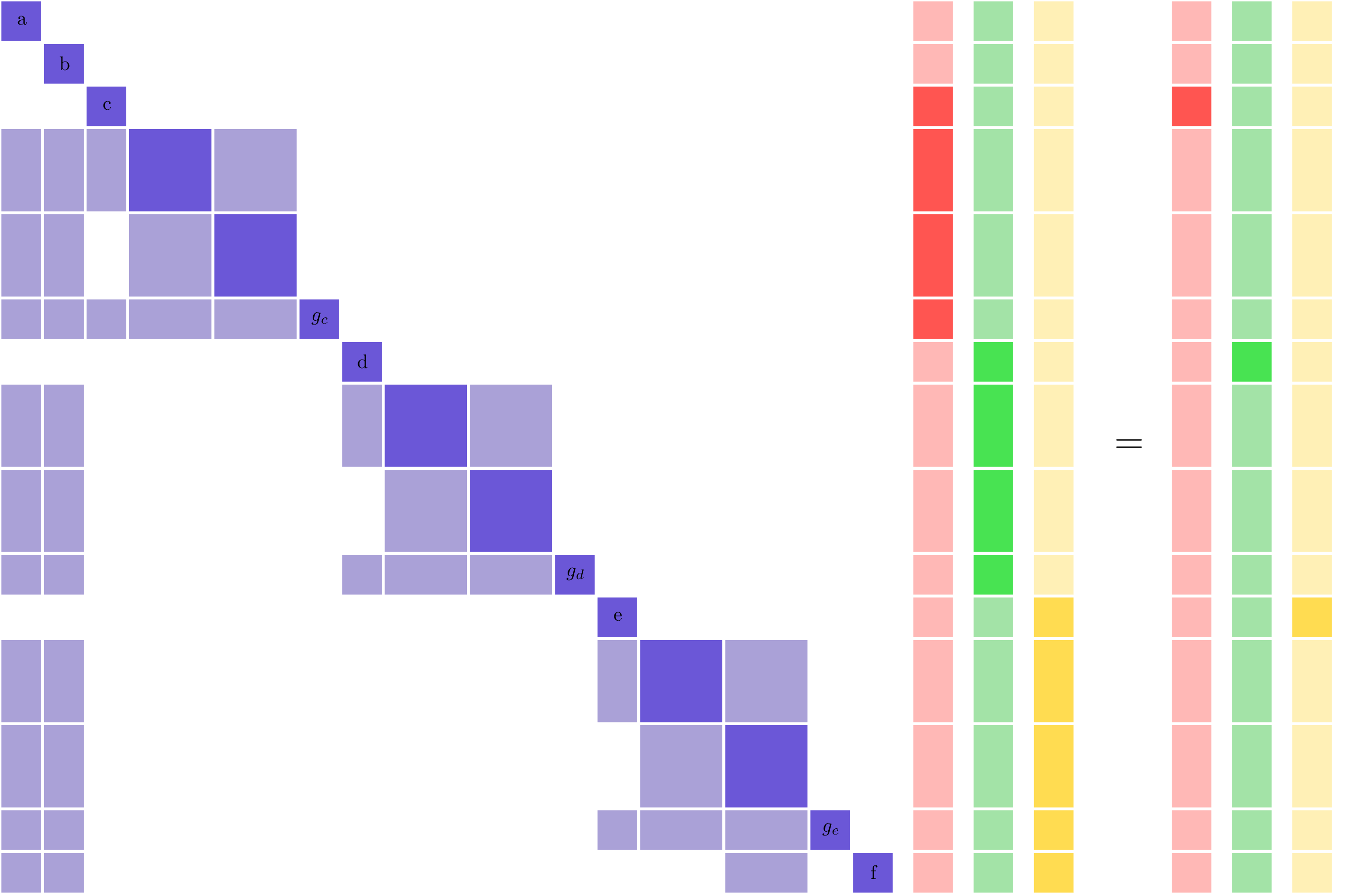
Those three solution vectors are non-overlapping because the three associated variables are separable. The forward-separable structure shows up clearly in the partial-derivative Jacobian, because it has been ordered to expose a block-diagonal structure. This allows us to collapse all three linear solves into a single simultaneous one:

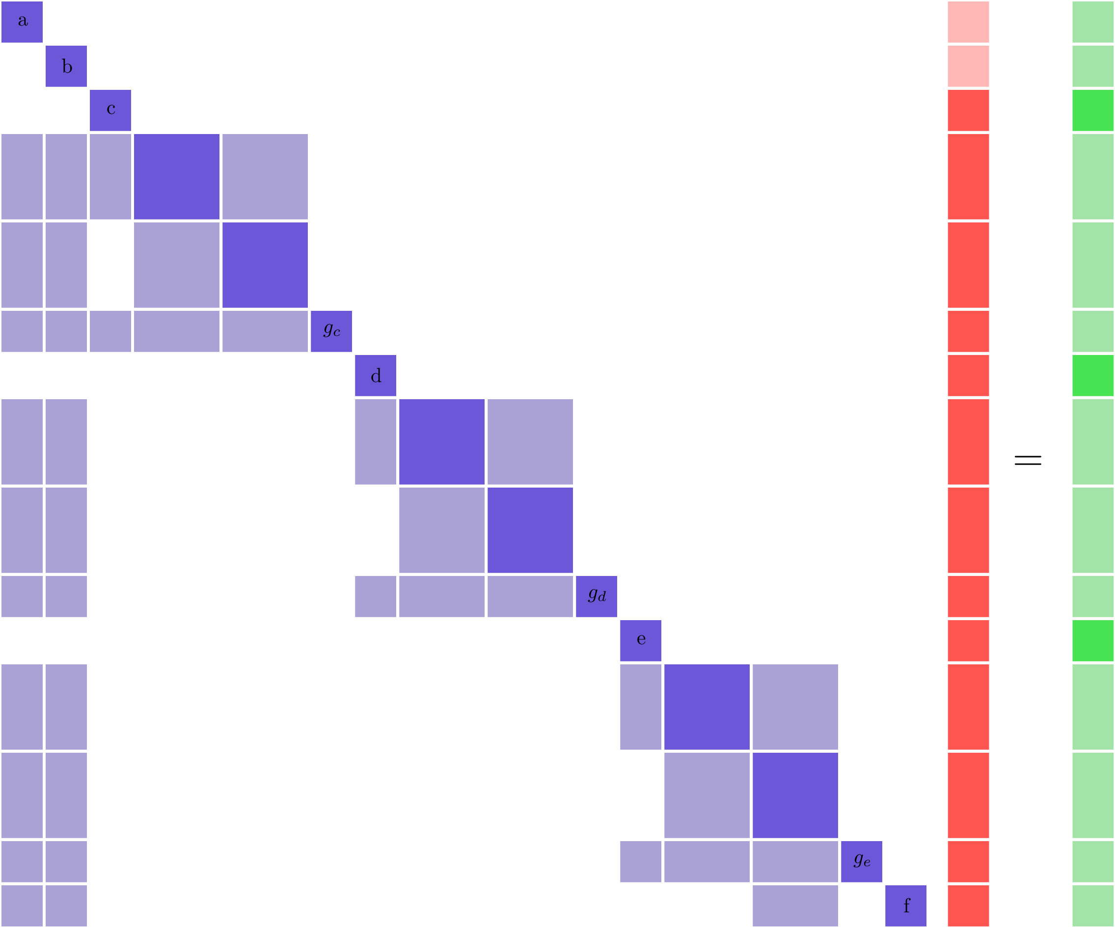
Using forward simultaneous derivatives reduces the required number of solves from 5 to 3 (2 for \(a, b\) and 1 for \(c, d, e\)). Hence, it would be faster to solve for total derivatives using forward mode with simultaneous derivatives than reverse mode.

Determining if Your Problem is Separable

The simple example above was contrived to make it relatively obvious that the problem was separable. For realistic problems, even if you know that the problem should be separable, computing the actual input/output sets can be challenging. You can think of the total derivative Jacobian as a graph with nodes representing each variable and non-zero entries representing edges connecting the nodes. Then the task of finding the separable variables can be performed using a graph-coloring algorithm. In that case, a set of separable variables are said to have the same color. The simple example problem would then have three colors; one each for \(a\) and \(b\) and one more for \(c,d,e\).

For any arbitrary problem, once you know the total-derivative Jacobian, then, in theory, you could color it. Since OpenMDAO can compute the total-derivative Jacobian, it would seem to be simply a matter of applying a coloring algorithm to it. However, there is a potential pitfall that needs to be accounted for. For any arbitrary point in the design space, some total derivatives could turn out to be zero, despite the fact that they are nonzero at other locations. An incidental zero would mean a missing edge in the graph, and could potentially deliver an incorrect coloring. The challenge is to figure out the non-zero entries in the total derivative Jacobian in a more robust way.

OpenMDAO knows the partial-derivative sparsity of a model because the nonzero partials are specified by each component in its setup method. So we need to compute the sparsity pattern of the total Jacobian, given the sparsity pattern of the partial Jacobian, in a way that reduces the chance of getting incidental zero values.

We can minimize the chance of having incidental zeros in the inverse by setting random numbers into the nonzero entries of the partial-derivative matrix, then computing the resulting total-derivative Jacobian using the randomized values. The derivatives computed in this way will not be physically meaningful, but the chance of having any incidental zero values is now very small. The likelihood of incidental zeros can be further reduced by computing the total-derivative Jacobian multiple times with different, random left-hand sides, and summing the absolute values of the resulting total-derivative Jacobians together.

Hence the cost of the coloring algorithm increases by the cost of \(n\) computations of the full total-derivative Jacobian. The larger you choose to make \(n\), the more reliable your coloring will be. If the model is intended to be used in an optimization context, then it is fair to assume that the total-derivative Jacobian is inexpensive enough to compute many times, and using a few additional computations to compute a coloring will not significantly impact the overall compute cost.

Choosing Forward or Reverse Mode for Separable Problems

If a problem has a section of design variables and constraints that are separable, then it is possible to leverage that quality in either forward or reverse mode. Which mode you choose depends on which direction gives you fewer total linear solves. In the example above, we show how separability changes the faster method from reverse to forward, but in general it does not have to cause that effect.

Normally you would count the number of design variables and responses and choose the mode corresponding to whichever one is smaller. For separable problems, you count the number of colors you have in each direction and choose which ever one is smaller. Sometimes the answer is different than you would get by counting design variables and constraints, but sometimes its not. The result is problem-dependent.

Relevance to Finite Difference and Complex Step

It is worth noting that, in addition to speeding up linear solutions for the unified derivative equations, forward separability also offers benefits when finite difference or complex step are being used to compute derivatives numerically. For the same reasons that multiple linear solves can be combined, you can also take steps in multiple variables to compute derivatives with respect to multiple variables at the same time.

How to actually use it!

OpenMDAO provides a mechanism for you to specify a coloring to take advantage of separability, via the use_fixed_coloring method. OpenMDAO also provides a coloring tool to determine the minimum number of colors your problem can be reduced to.

You can also see an example of setting up an optimization with simultaneous derivatives in the Simple Optimization using Simultaneous Derivatives example.