Finding Feasible Solutions

Constrained, gradient-based optimization tools like SLSQP, IPOPT, and SNOPT can benefit from starting from a feasible design point, but finding a feasible design with dozens or hundreds of design variables can be a challenge in itself.

Domain-specific methods exist for finding a feasible starting point, such as using a suboptimal explicit simulation to jump-start an implicit trajectory optimization, but in a multidisciplinary environment a more general approach is needed.

OpenMDAO’s Problem.find_feasible method aims to find a feasible point if one exists, or otherwise minimize the violation of infeasible constraints in the design.

This approach poses the constraint violations as residuals to be minimized via a least-squares approach. Under the hood, it utilizes scipy.optimize.least_squares to perform this minimization.

Problem.find_feasible(case_prefix=None, reset_iter_counts=True, driver_scaling=True, exclude_desvars=None, method='trf', ftol=1e-08, xtol=1e-08, gtol=1e-08, x_scale=1.0, loss='linear', loss_tol=1e-08, f_scale=1.0, max_nfev=None, tr_solver=None, tr_options=None, iprint=1)

Attempt to find design variable values which minimize the constraint violation.

If the problem is feasible, this method should find the solution for which the violation of each constraint is zero.

This approach uses a least-squares minimization of the constraint violation. If the problem has a feasible solution, this should find the feasible solution closest to the current design variable values.

Arguments method, ftol, xtol, gtol, x_scale, loss, f_scale, diff_step, tr_solver, tr_options, and verbose are passed to scipy.optimize.least_squares, see the documentation of that function for more information: https://docs.scipy.org/doc/scipy/reference/generated/scipy.optimize.least_squares.html

Parameters:

case_prefixstr or None

Prefix to prepend to coordinates when recording. None means keep the preexisting prefix.

reset_iter_countsbool

If True and model has been run previously, reset all iteration counters.

driver_scalingbool

If True, consider the constraint violation in driver-scaled units. Otherwise, it will be computed in the model’s units.

exclude_desvarsstr or Sequence[str] or None

If given, a pattern of one or more design variables to be excluded from the least-squares search. The allows for finding a feasible (or least infeasible) solution when holding one or more design variables to their current values.

method{‘trf’, ‘dogbox’, or ‘lm’}

The method used by scipy.optimize.least_squares. One or ‘trf’, ‘dogbox’, or ‘lm’.

ftolfloat or None

The change in the cost function from one iteration to the next which triggers a termination of the minimization.

xtolfloat or None

The change in the design variable vector norm from one iteration to the next which triggers a termination of the minimization.

gtolfloat or None

The change in the gradient norm from one iteration to the next which triggers a termination of the minimization.

x_scale{float, array-like, or ‘jac’}

Additional scaling applied by the least-squares algorithm. Behavior is method-dependent. For additional details, see the scipy documentation.

loss{‘linear’, ‘soft_l1’, ‘huber’, ‘cauchy’, or ‘arctan’}

The loss aggregation method. Options of interest are: - ‘linear’ gives the standard “sum-of-squares”. - ‘soft_l1’ gives a smooth approximation for the L1-norm of constraint violation. For other options, see the scipy documentation.

loss_tolfloat

The tolerance on the loss value above which the algorithm is considered to have failed to find a feasible solution. This will result in the DriverResult.success attribute being False, and this method will return as _failed_.

f_scalefloat or None

Value of margin between inlier and outlier residuals when loss is not ‘linear’. For more information, see the scipy documentation.

max_nfevint or None

The maximum allowable number of model evaluations. If not provided scipy will determine it automatically based on the size of the design variable vector.

tr_solver{None, ‘exact’, or ‘lsmr’}

The solver used by trust region (trf) method. For more details, see the scipy documentation.

tr_optionsdict or None

Additional options for the trust region (trf) method. For more details, see the scipy documentation.

iprintint

Verbosity of the output. Use 2 for the full verbose least_squares output. Use 1 for a convergence summary, and 0 to suppress output.

Returns:

bool

Failure flag; True if failed to converge, False is successful.

Consider the following optimization problem. It contains two constraints which are in conflict with each other.

()\[\begin{align} \mathrm{Minimize}: \\ y = x_1^2 - x_2^2 \\ \mathrm{Subject\,to:} \\ g_1 = 2 x_1 - 5 \\ g_2 = -2 x_1 - 5 \\ g_3 = x_2 - 5 \end{align}\]

The OpenMDAO problem can be formulated as follows:

import numpy as np
import openmdao.api as om

prob = om.Problem()

c1 = om.ExecComp()
c1.add_expr('y = x1**2 - x2**2', y={'copy_shape': 'x1'}, x1={'shape_by_conn': True}, x2={'shape_by_conn': True})
c1.add_expr('g1 = 2 * x1 - 5', g1={'copy_shape': 'x1'})
c1.add_expr('g2 = -2 * x1 - 5', g2={'copy_shape': 'x1'})
c1.add_expr('g3 = x2 - 5', g3={'copy_shape': 'x2'})

c1.add_design_var('x1', lower=-10, upper=10)
c1.add_design_var('x2', lower=-10, upper=10)
c1.add_objective('y')
c1.add_constraint('g1', lower=0)
c1.add_constraint('g2', lower=0)
c1.add_constraint('g3', lower=0)

prob.model.add_subsystem('c1', c1, promotes=['*'])
prob.driver = om.ScipyOptimizeDriver()

The feasible regions due to each constraint are shaded in the figure below. Note that there is no solution which satisfies all three constraints.

Show code cell source Hide code cell source

%matplotlib inline

import matplotlib.pyplot as plt

x1s = np.linspace(-10, 10, 100)
x2s = np.linspace(-10, 10, 100)
xx1, xx2 = np.meshgrid(x1s, x2s)

prob.setup()
prob.set_val('x1', xx1)
prob.set_val('x2', xx2)

prob.run_model()

ys = prob.get_val('y')

fig, ax = plt.subplots(1, 1, figsize=(8, 6))
ax.contour(x1s, x2s, ys, levels=20)
ax.fill_between(np.linspace(-10, 10, 10), 5 * np.ones(10), 10 * np.ones(10), color='r', alpha=0.3)
ax.fill_between(np.linspace(2.5, 10, 10), -10 * np.ones(10), 10 * np.ones(10), color='g', alpha=0.3)
ax.fill_between(np.linspace(-10, -2.5, 10), -10 * np.ones(10), 10 * np.ones(10), color='b', alpha=0.3)
ax.set_xlabel('$x_1$')
ax.set_ylabel('$x_2$')
ax.grid()
plt.show()

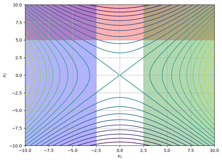
If we perform an optimization with the driver, it will fail due to the incompatible constraints.

# Call setup again so we can use a new size for x1 and x2
prob.setup()

prob.set_val('x1', 1.0)
prob.set_val('x2', 1.0)

prob.run_driver()
prob.list_driver_vars(cons_opts=['lower', 'upper'], objs_opts=['val']);

Positive directional derivative for linesearch    (Exit mode 8)
            Current function value: -99.00000000001629
            Iterations: 27
            Function evaluations: 221
            Gradient evaluations: 23
Optimization FAILED.
Positive directional derivative for linesearch
-----------------------------------
----------------
Design Variables
----------------
name  val    size  lower  upper  ref   ref0  indices  adder  scaler  parallel_deriv_color  cache_linear_solution  units  
----  -----  ----  -----  -----  ----  ----  -------  -----  ------  --------------------  ---------------------  ----- 
x1    [1.]   1     -10.0  10.0   None  None  None     None   None    None                  False                  None   
x2    [10.]  1     -10.0  10.0   None  None  None     None   None    None                  False                  None   

-----------
Constraints
-----------
name  val    size  indices  alias  lower  upper  
----  -----  ----  -------  -----  -----  ----- 
g1    [-3.]  1     None     None   0.0    1e+30  
g2    [-7.]  1     None     None   0.0    1e+30  
g3    [5.]   1     None     None   0.0    1e+30  

----------
Objectives
----------
name  val     size  indices  
----  ------  ----  ------- 
y     [-99.]  1     None     

/usr/share/miniconda/envs/test/lib/python3.12/site-packages/openmdao/utils/coloring.py:447: DerivativesWarning:'c1' <class ExecComp>: Coloring was deactivated.  Improvement of 0.0% was less than min allowed (5.0%).

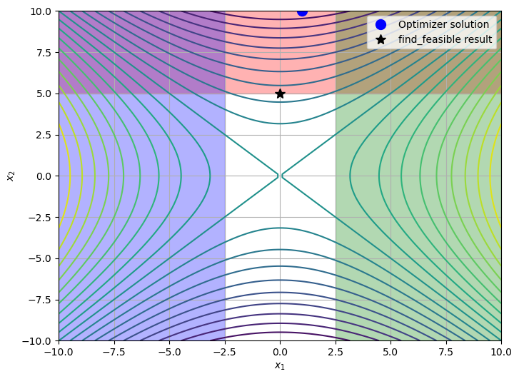
If we use the find_feasible method on Problem, we can find the solution which minimizes the L2 norm of the constraint violations. This method will attempt to find the solution that minimizes the constraint violations. If it fails to converge to a solution, it will return as having failed. If it converges but the solution is still infeasible (it found the solution which minimizes the constraint violation), it will also return as having failed.

x1_opt = prob.get_val('x1').copy()
x2_opt = prob.get_val('x2').copy()

prob.set_val('x1', 1.0)
prob.set_val('x2', 1.0)

prob.find_feasible()
prob.list_driver_vars(desvar_opts=['lower', 'upper'], cons_opts=['lower', 'upper'], objs_opts=['val']);

-------------------------
Infeasibilities minimized
-------------------------
    loss(linear): 25.00000000
    iterations: 7
    model evals: 7
    gradient evals: 7
    elapsed time: 0.00351752 s
    max violation: g1[0] = -5.00000000

----------------
Design Variables
----------------
name  val                size  indices  lower  upper  
----  -----------------  ----  -------  -----  ----- 
x1    [-2.93033752e-16]  1     None     -10.0  10.0   
x2    [5.]               1     None     -10.0  10.0   

-----------
Constraints
-----------
name  val                size  indices  alias  lower  upper  
----  -----------------  ----  -------  -----  -----  ----- 
g1    [-5.]              1     None     None   0.0    1e+30  
g2    [-5.]              1     None     None   0.0    1e+30  
g3    [-3.99680289e-14]  1     None     None   0.0    1e+30  

----------
Objectives
----------
name  val     size  indices  
----  ------  ----  ------- 
y     [-25.]  1     None     

The following plot highlights the difference between the solution at the end of the failed optimization run, versus the solution found which minimizes feasibilities.

Show code cell source Hide code cell source

x1_min_infeas = prob.get_val('x1').copy()
x2_min_infeas = prob.get_val('x2').copy()

fig, ax = plt.subplots(1, 1, figsize=(8, 6))
ax.contour(x1s, x2s, ys, levels=20)
ax.fill_between(np.linspace(-10, 10, 10), 5 * np.ones(10), 10 * np.ones(10), color='r', alpha=0.3)
ax.fill_between(np.linspace(2.5, 10, 10), -10 * np.ones(10), 10 * np.ones(10), color='g', alpha=0.3)
ax.fill_between(np.linspace(-10, -2.5, 10), -10 * np.ones(10), 10 * np.ones(10), color='b', alpha=0.3)
ax.plot(x1_opt, x2_opt, 'bo', ms=10, label='Optimizer solution')
ax.plot(x1_min_infeas, x2_min_infeas, 'k*', ms=10, label='find_feasible result')
ax.set_xlabel('$x_1$')
ax.set_ylabel('$x_2$')
ax.grid()
ax.legend()
plt.show()

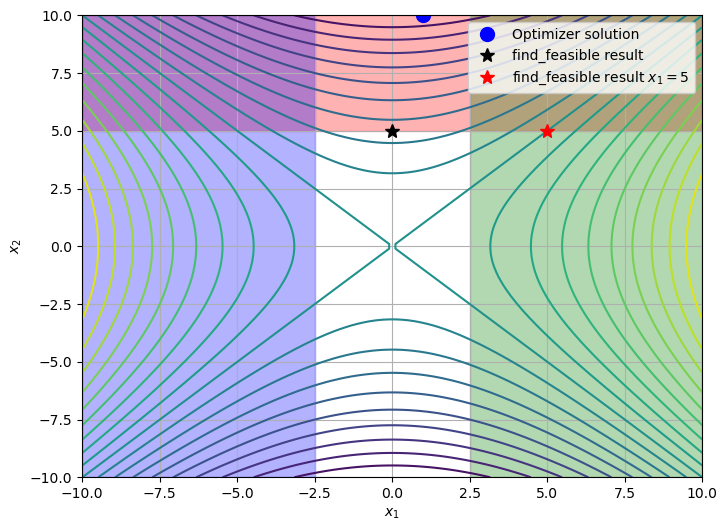
Omitting one or more design variables from the feasibility search

Sometimes the user may be interested in finding a feasible (or least infeasible) solution at a given value of one or more design variables. The find_feasible method supports an exclude_desvars keyword argument that allows the user to exclude one or more design variables from the feasibility search. This argument may be a glob pattern which can match one or more design variable names.

For instance, let’s find the minimimum-infeasibility-solution such that \(x_1 = 5\).

prob.set_val('x1', 5.0)

prob.find_feasible(exclude_desvars=['x1'])
prob.list_driver_vars(desvar_opts=['lower', 'upper'], cons_opts=['lower', 'upper'], objs_opts=['val']);

-------------------------
Infeasibilities minimized
-------------------------
    loss(linear): 112.50000000
    iterations: 1
    model evals: 1
    gradient evals: 1
    elapsed time: 0.00112365 s
    max violation: g2[0] = -15.00000000

----------------
Design Variables
----------------
name  val   size  indices  lower  upper  
----  ----  ----  -------  -----  ----- 
x1    [5.]  1     None     -10.0  10.0   
x2    [5.]  1     None     -10.0  10.0   

-----------
Constraints
-----------
name  val                size  indices  alias  lower  upper  
----  -----------------  ----  -------  -----  -----  ----- 
g1    [5.]               1     None     None   0.0    1e+30  
g2    [-15.]             1     None     None   0.0    1e+30  
g3    [-3.99680289e-14]  1     None     None   0.0    1e+30  

----------
Objectives
----------
name  val               size  indices  
----  ----------------  ----  ------- 
y     [3.97903932e-13]  1     None     

Show code cell source Hide code cell source

x1_min_infeas_x1_fixed = prob.get_val('x1').copy()
x2_min_infeas_x1_fixed = prob.get_val('x2').copy()

fig, ax = plt.subplots(1, 1, figsize=(8, 6))
ax.contour(x1s, x2s, ys, levels=20)
ax.fill_between(np.linspace(-10, 10, 10), 5 * np.ones(10), 10 * np.ones(10), color='r', alpha=0.3)
ax.fill_between(np.linspace(2.5, 10, 10), -10 * np.ones(10), 10 * np.ones(10), color='g', alpha=0.3)
ax.fill_between(np.linspace(-10, -2.5, 10), -10 * np.ones(10), 10 * np.ones(10), color='b', alpha=0.3)
ax.plot(x1_opt, x2_opt, 'bo', ms=10, label='Optimizer solution')
ax.plot(x1_min_infeas, x2_min_infeas, 'k*', ms=10, label='find_feasible result')
ax.plot(x1_min_infeas_x1_fixed, x2_min_infeas_x1_fixed, 'r*', ms=10, label='find_feasible result $x_1=5$')
ax.set_xlabel('$x_1$')
ax.set_ylabel('$x_2$')
ax.grid()
ax.legend()
plt.show()