Instance-based Profiling

Instance-based Profiling#

Python has several good profilers available for general python code, and instance-based profiling is not meant to replace general profiling. However, because the OpenMDAO profiler lets you view the profiled functions grouped by the specific Problem, System, Group, Driver, or Solver that called them, it can provide insight into which parts of your model are more expensive, even when different parts of your model use many of the same underlying functions.

Instance-based profiling by default will record information for all calls to any of the main OpenMDAO classes or their descendants, for example, System, Problem, Solver, Driver, Matrix and Jacobian.

The simplest way to use instance-based profiling is via the command line using the openmdao iprof command. For example:

    openmdao iprof <your_python_script_here>

This will collect the profiling data, start a web server, and pop up an icicle viewer in a web browser.

Generally it’s best to just use all of the defaults, but if necessary you can change the server port number using the -p option, or change the title of the displayed page using the -t option, for example:

    openmdao iprof <your_python_script_here> -p 8801 -t "Instance Profile for propulsor.py"

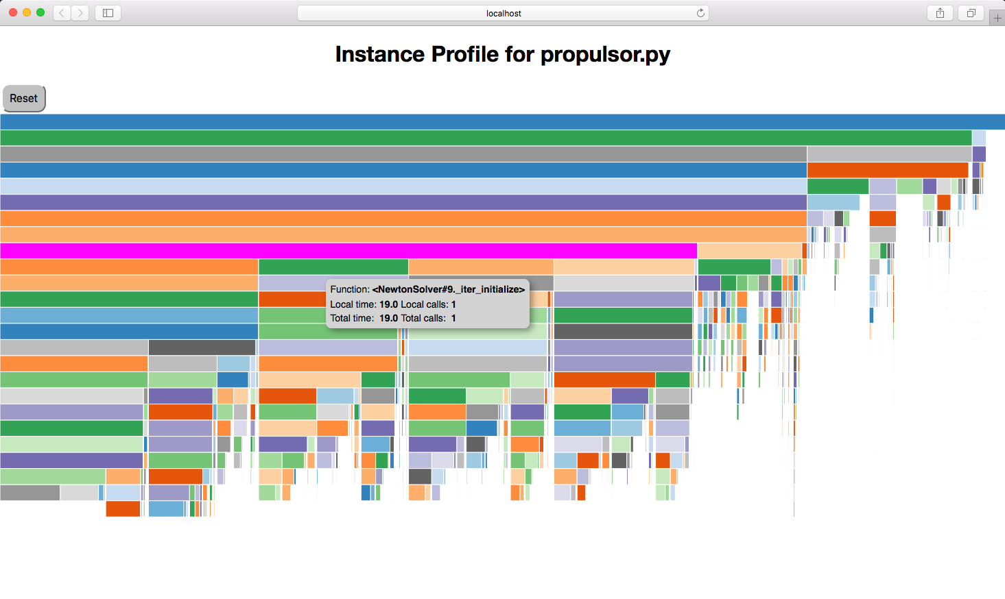
You should then see something like this: An example of a profile icicle viewer

In the viewer, hovering over a box will show the function pathname, the local and total elapsed time for that function, and the local and total number of calls for that function. Clicking on a box will collapse the view so that that box’s function will become the top box and only functions called by that function will be visible. The top box before any box has been collapsed is called $total and does not represent a real function. Instead, it shows the total time that profiling was active. If there are gaps below a parent block, i.e. its child blocks don’t cover the entire space below the parent, that gap represents the time exclusive to the parent or time taken up by functions called by the parent that are not being profiled.

There is a Reset button that will take you back to the top level of the profile after you have clicked down into a sub-call.

Documentation of options for all commands described here can be obtained by running the command followed by the -h option. For example:

    openmdao iprof -h

usage: openmdao iprof [-h] [-p PORT] [--no_browser] [-t TITLE] [-g METHODS] [-m MAXCALLS] file [file ...]

positional arguments:
  file                  Raw profile data files or a python file.

optional arguments:
  -h, --help            show this help message and exit
  -p PORT, --port PORT  port used for web server
  --no_browser          Don't pop up a browser to view the data.
  -t TITLE, --title TITLE
                        Title to be displayed above profiling view.
  -g METHODS, --group METHODS
                        Determines which group of methods will be tracked. Current options are: ['coloring', 'dataflow', 'driver',
                        'jac', 'linear', 'openmdao', 'openmdao_all', 'setup', 'solver', 'transfer'] and "openmdao" is the default
  -m MAXCALLS, --maxcalls MAXCALLS
                        Maximum number of calls displayed at one time. Default=15000.

If you just want to see the timing totals for each method, you can call openmdao iprof_totals instead of openmdao iprof. For example:

    openmdao iprof_totals <your_python_script_here>

openmdao iprof_totals will write tabular output to the terminal containing total runtime and total number of calls for each profiled function. For example:

Total     Total           Function
Calls     Time (s)    %   Name
  0.000000   0.00 des_vars.<System.initialize>
  0.000000   0.00 <Solver#3._declare_options>
  0.000000   0.00 <Solver#6._declare_options>
  0.000000   0.00 <Solver#7._declare_options>
  0.000000   0.00 <Solver#9._declare_options>
  0.000000   0.00 <Solver#15._declare_options>
  0.000000   0.00 design.fc.ambient.<System.initialize>
  0.000000   0.00 <Solver#16._declare_options>
  0.000000   0.00 design.fc.conv.<System.initialize>
  0.000000   0.00 <Solver#20._declare_options>
  0.000000   0.00 <Solver#21._declare_options>
  0.000000   0.00 <Solver#25._declare_options>
  0.000000   0.00 design.fc.ambient.readAtmTable.<System.initialize>
   ...
  1.690505   8.06 <NonlinearRunOnce#5.solve>
  1.694799   8.08 design.fc.conv.fs.exit_static.<Group._solve_nonlinear>
  1.885014   8.99 <NonlinearRunOnce#6.solve>
  1.892510   9.02 design.fc.conv.fs.<Group._solve_nonlinear>
  1.934901   9.23 .<System._setup_scaling>
  2.053042   9.79 design.fan.<Group._setup_vars>
  2.549496  12.16 <NewtonSolver#2._iter_execute>
  2.609760  12.44 <Solver#22._run_iterator>
  2.609783  12.44 <NonlinearSolver#2.solve>
  2.613209  12.46 design.fc.conv.<Group._solve_nonlinear>
  2.615414  12.47 <NonlinearRunOnce#7.solve>
  2.619340  12.49 design.fc.<Group._solve_nonlinear>
  3.133403  14.94 design.nozz.<Group._setup_vars>
  7.319256  34.90 <NewtonSolver#1._iter_execute>
  7.608798  36.28 <Solver#13._run_iterator>
  7.608808  36.28 <NonlinearSolver#1.solve>
  7.617416  36.32 design.<Group._solve_nonlinear>
  7.617761  36.32 <NonlinearRunOnce#32.solve>
  7.627209  36.37 .<Group._solve_nonlinear>
  7.627431  36.37 .<System.run_solve_nonlinear>
  7.627438  36.37 <Problem#1.run_model>
  7.818091  37.28 design.<Group._setup_vars>
  7.863608  37.49 .<Group._setup_vars>
 12.812045  61.09 .<System._setup>
 12.826367  61.16 <Problem#1.setup>
 20.973087 100.00 $total

Note that the totals are sorted with the largest values at the end so that when running openmdao iprof_totals in a terminal the most important functions will show up without having to scroll to the top of the output, which can be lengthy. Also note that the function names are a combination of the OpenMDAO pathname (when available) plus the function name qualified by the owning class, or the class name followed by an instance identifier, plus the function name.

Note

Running either openmdao iprof or openmdao iprof_totals will generate by default a file called iprof.0 in your current directory. Either script can be run directly on the iprof.0 file and will generate the same outputs as running your python script.

If you want more control over the profiling process, you can import openmdao.devtools.iprofile and manually call setup(), start() and stop(). For example:

from openmdao.devtools import iprofile

# we'll just use defaults here, but we could change the methods to profile in the call to setup()
iprofile.setup()
iprofile.start()

# define my model and run it...

iprofile.stop()

# do some other stuff that I don't want to profile...

After your script is finished running, you should see a new file called iprof.0 in your current directory. If you happen to have activated profiling for an MPI run, then you’ll have a copy of that file for each MPI process, so iprof.0, iprof.1, etc. As mentioned earlier, you can run either openmdao iprof or openmdao iprof_totals directly on the iprof.* data file(s).

Warning

The timing numbers obtained from instance-based profiling will not be exact due to overhead introduced by the python function that collects timing data.

Warning

If your script contains any quit() or exit() calls, it will cause the profiling to fail because the profiling performs certain necessary operations in a function registered with atexit. This function will not execute if a quit() or exit() is encountered.