Visually Checking Partial Derivatives with Matrix Diagrams

The function partial_deriv_plot lets you see a visual representation of the values returned by check_partials.

openmdao.visualization.partial_deriv_plot.partial_deriv_plot(of, wrt, check_partials_data, title=None, jac_method='J_fwd', tol=1e-10, binary=True)

Visually examine the computed and finite differenced Jacobians.

Parameters:

ofstr

Variable whose derivatives will be computed.

wrtstr

Variable with respect to which the derivatives will be computed.

check_partials_datadict of dicts of dicts

First key:

is the component name;

Second key:

is the (output, input) tuple of strings;

Third key:

is one of [‘rel error’, ‘abs error’, ‘magnitude’, ‘J_fd’, ‘J_fwd’, ‘J_rev’];

For ‘rel error’, ‘abs error’, ‘magnitude’ the value is: A tuple containing norms for

forward - fd, adjoint - fd, forward - adjoint.

For ‘J_fd’, ‘J_fwd’, ‘J_rev’ the value is: A numpy array representing the computed

Jacobian for the three different methods of computation.

titlestr (Optional)

Title for the plot If None, use the values of the arguments “of” and “wrt”.

jac_methodstr (Optional)

Method of computating Jacobian Is one of [‘J_fwd’, ‘J_rev’]. Optional, default is ‘J_fwd’.

tolfloat (Optional)

The tolerance, below which the two numbers are considered the same for plotting purposes.

binarybool (Optional)

If true, the plot will only show the presence of a non-zero derivative, not the value. Otherwise, plot the value. Default is true.

Returns:

matplotlib.figure.Figure

The top level container for all the plot elements in the plot.

array of matplotlib.axes.Axes objects

An array of Axes objects, one for each of the three subplots created.

Raises:

KeyError

If one of the Jacobians is not available.

Here are two examples of its use. Note that in these examples, the compute_partials method intentionally computes the incorrect value so that the plots show how this function can be used to detect such errors.

With the default value of binary equal to True, the plots will only show the presence of a non-zero derivative, not the value.

import numpy as np
import openmdao.api as om

class ArrayComp2D(om.ExplicitComponent):
    """
    A fairly simple array component with an intentional error in compute_partials.
    """
    def setup(self):
        self.JJ = np.array([[1.0, 0.0, 0.0, 7.0],
                            [0.0, 2.5, 0.0, 0.0],
                            [-1.0, 0.0, 8.0, 0.0],
                            [0.0, 4.0, 0.0, 6.0]])
        # Params
        self.add_input('x1', np.ones([4]))
        # Unknowns
        self.add_output('y1', np.zeros([4]))
        self.declare_partials(of='*', wrt='*')

    def compute(self, inputs, outputs):
        """
        Execution.
        """
        outputs['y1'] = self.JJ.dot(inputs['x1'])

    def compute_partials(self, inputs, partials):
        """
        Analytical derivatives.
        """
        # create some error to force the diff plot to show something
        error = np.zeros((4, 4))
        err = 1e-7
        error[0][3] = err
        error[1][2] = - 2.0 * err
        partials[('y1', 'x1')] = self.JJ + error

prob = om.Problem()
model = prob.model
model.add_subsystem('mycomp', ArrayComp2D(), promotes=['x1', 'y1'])
prob.setup(check=False, mode='fwd')
check_partials_data = prob.check_partials(out_stream=None)

# plot with defaults
om.partial_deriv_plot('y1', 'x1', check_partials_data)

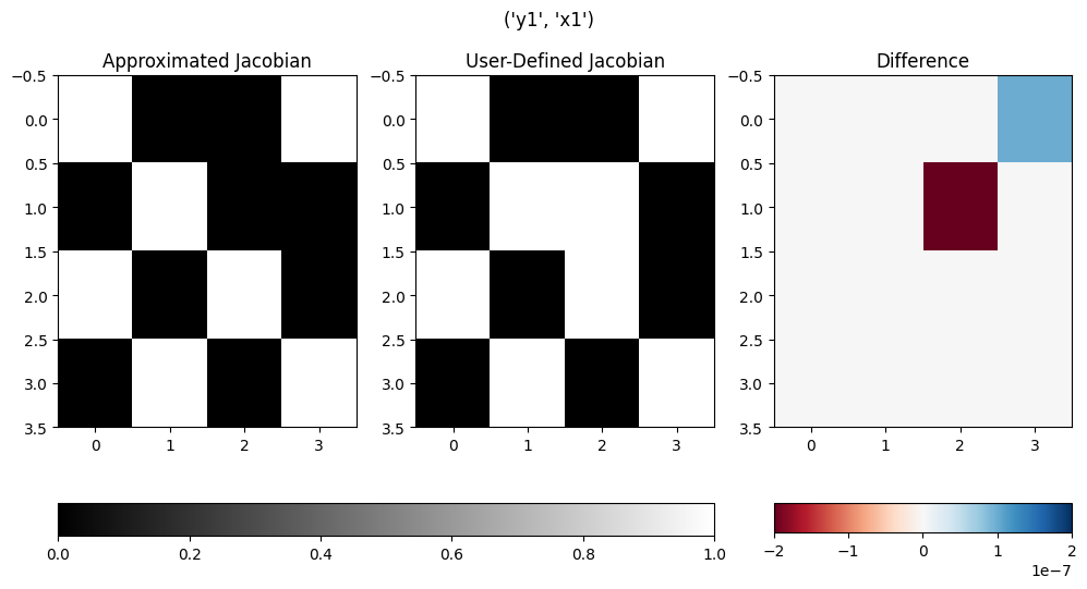
(<Figure size 1200x600 with 5 Axes>,
 array([<Axes: title={'center': 'Approximated Jacobian'}>,
        <Axes: title={'center': 'User-Defined Jacobian'}>,
        <Axes: title={'center': 'Difference'}>], dtype=object))

With the value of binary equal to False, the plots show the actual value.

import numpy as np
import openmdao.api as om

class ArrayComp2D(om.ExplicitComponent):
    """
    A fairly simple array component with an intentional error in compute_partials.
    """
    def setup(self):
        self.JJ = np.array([[1.0, 0.0, 0.0, 7.0],
                            [0.0, 2.5, 0.0, 0.0],
                            [-1.0, 0.0, 8.0, 0.0],
                            [0.0, 4.0, 0.0, 6.0]])
        # Params
        self.add_input('x1', np.ones([4]))
        # Unknowns
        self.add_output('y1', np.zeros([4]))
        self.declare_partials(of='*', wrt='*')

    def compute(self, inputs, outputs):
        """
        Execution.
        """
        outputs['y1'] = self.JJ.dot(inputs['x1'])

    def compute_partials(self, inputs, partials):
        """
        Analytical derivatives.
        """
        # create some error to force the diff plot to show something
        error = np.zeros((4, 4))
        err = 1e-7
        error[0][3] = err
        error[1][2] = - 2.0 * err
        partials[('y1', 'x1')] = self.JJ + error

prob = om.Problem()
model = prob.model
model.add_subsystem('mycomp', ArrayComp2D(), promotes=['x1', 'y1'])
prob.setup(check=False, mode='fwd')
check_partials_data = prob.check_partials(out_stream=None)

# plot in non-binary mode
om.partial_deriv_plot('y1', 'x1', check_partials_data, binary = False)

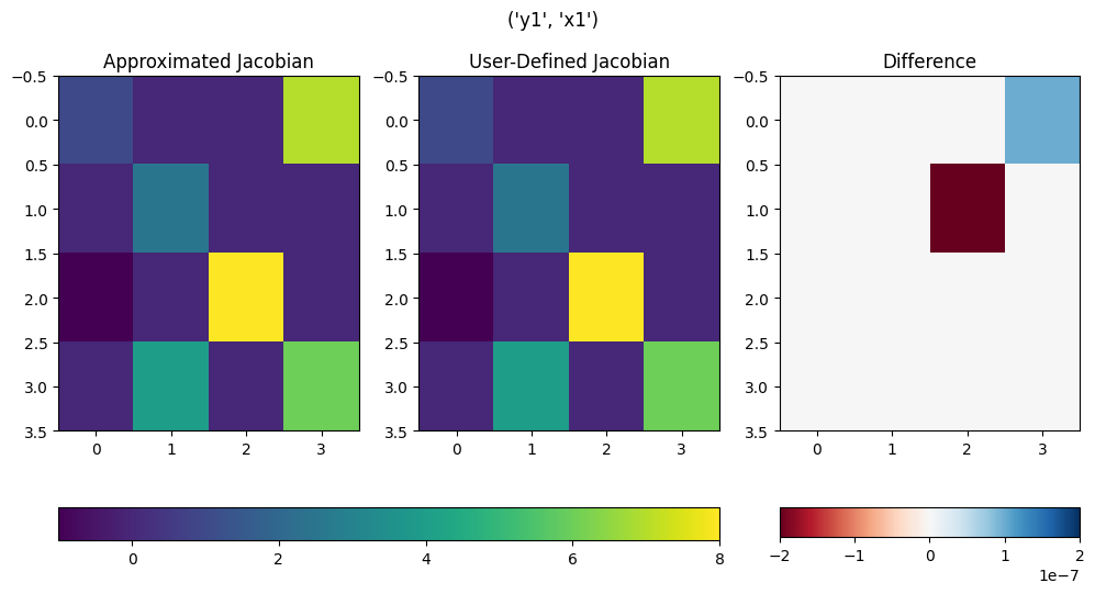
(<Figure size 1200x600 with 5 Axes>,
 array([<Axes: title={'center': 'Approximated Jacobian'}>,
        <Axes: title={'center': 'User-Defined Jacobian'}>,
        <Axes: title={'center': 'Difference'}>], dtype=object))