Composable functions via jax (openmdao.jax)

Certain functions are useful in a gradient-based optimization context, such as smooth activation functions or differentiable maximum/minimum functions.

Rather than provide a component that forces a user to structure their system in a certain way and add more components than necessary, the openmdao.jax package is intended to provide a universal source for composable functions that users can use within their own components.

Functions in openmdao.jax are built using the jax Python package. This allows users to develop components that use these functions, along with other code written with jax, and leverage capabilities of jax like automatic differentiation, vectorization, and just-in-time compilation. For most users, these functions will be used within the compute_primal method of a JaxExplicitComponent or JaxImplicitComponent, but users who are proficient in jax can also write their own custom components using these functions if necessary.

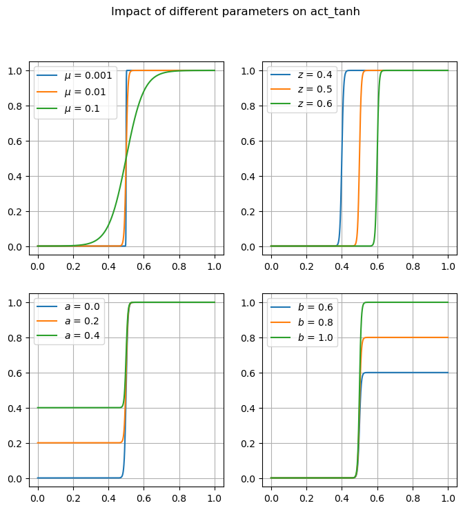
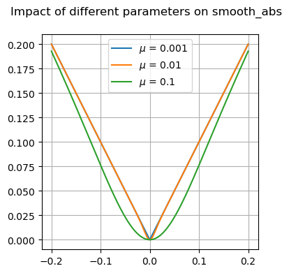
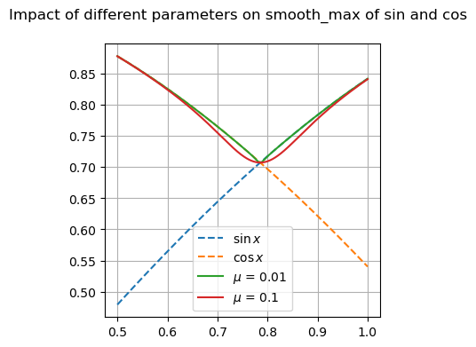
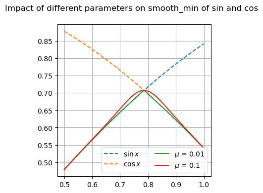
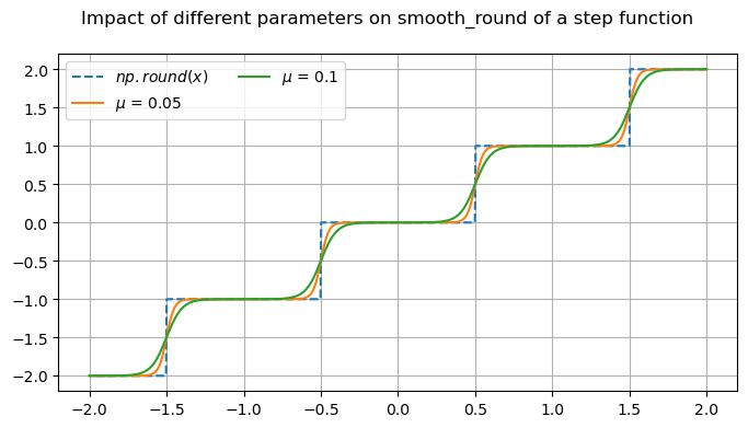
Many of these functions are focused on providing differentiable forms of strictly non-differentiable functions, such as step responses, absolute value, and minimums or maximums. Near regions where the nominal functions would have invalid derivatives, these functions are smooth but will not perfectly match their non-smooth counterparts.

Available Functions

Show code cell source

Hide code cell source

import numpy as np
import matplotlib.pyplot as plt
import openmdao.jax_funcs as omj

fig, ax = plt.subplots(2, 2, figsize=(8, 8))
fig.suptitle('Impact of different parameters on act_tanh')
x = np.linspace(0, 1, 1000)

mup001 = omj.act_tanh(x, mu=0.001, z=0.5, a=0, b=1)
mup01 = omj.act_tanh(x, mu=0.01, z=0.5, a=0, b=1)
mup1 = omj.act_tanh(x, mu=0.1, z=0.5, a=0, b=1)

ax[0, 0].plot(x, mup001, label=r'$\mu$ = 0.001')
ax[0, 0].plot(x, mup01, label=r'$\mu$ = 0.01')
ax[0, 0].plot(x, mup1, label=r'$\mu$ = 0.1')
ax[0, 0].legend()
ax[0, 0].grid()

zp5 = omj.act_tanh(x, mu=0.01, z=0.5, a=0, b=1)
zp4 = omj.act_tanh(x, mu=0.01, z=0.4, a=0, b=1)
zp6 = omj.act_tanh(x, mu=0.01, z=0.6, a=0, b=1)

ax[0, 1].plot(x, zp4, label=r'$z$ = 0.4')
ax[0, 1].plot(x, zp5, label=r'$z$ = 0.5')
ax[0, 1].plot(x, zp6, label=r'$z$ = 0.6')
ax[0, 1].legend()
ax[0, 1].grid()

a0 = omj.act_tanh(x, mu=0.01, z=0.5, a=0, b=1)
ap2 = omj.act_tanh(x, mu=0.01, z=0.5, a=0.2, b=1)
ap4 = omj.act_tanh(x, mu=0.01, z=0.5, a=0.4, b=1)

ax[1, 0].plot(x, a0, label=r'$a$ = 0.0')
ax[1, 0].plot(x, ap2, label=r'$a$ = 0.2')
ax[1, 0].plot(x, ap4, label=r'$a$ = 0.4')
ax[1, 0].legend()
ax[1, 0].grid()

bp6 = omj.act_tanh(x, mu=0.01, z=0.5, a=0, b=.6)
bp8 = omj.act_tanh(x, mu=0.01, z=0.5, a=0, b=.8)
b1 = omj.act_tanh(x, mu=0.01, z=0.5, a=0, b=1)

ax[1, 1].plot(x, bp6, label=r'$b$ = 0.6')
ax[1, 1].plot(x, bp8, label=r'$b$ = 0.8')
ax[1, 1].plot(x, b1, label=r'$b$ = 1.0')
ax[1, 1].legend()
ax[1, 1].grid()

Show code cell source

Hide code cell source

fig, ax = plt.subplots(1, 1, figsize=(4, 4))
fig.suptitle('Impact of different parameters on smooth_abs')
x = np.linspace(-0.2, 0.2, 1000)

mup001 = omj.smooth_abs(x, mu=0.001)
mup01 = omj.smooth_abs(x, mu=0.01)
mup1 = omj.smooth_abs(x, mu=0.1)

ax.plot(x, mup001, label=r'$\mu$ = 0.001')
ax.plot(x, mup01, label=r'$\mu$ = 0.01')
ax.plot(x, mup1, label=r'$\mu$ = 0.1')
ax.legend()
ax.grid()

Show code cell source

Hide code cell source

fig, ax = plt.subplots(1, 1, figsize=(4, 4))
fig.suptitle('Impact of different parameters on smooth_max of sin and cos')
x = np.linspace(0.5, 1, 1000)

sin = np.sin(x)
cos = np.cos(x)

mup001 = omj.smooth_max(sin, cos, mu=0.001)
mup01 = omj.smooth_max(sin, cos, mu=0.01)
mup1 = omj.smooth_max(sin, cos, mu=0.1)

ax.plot(x, sin, '--', label=r'$\sin{x}$')
ax.plot(x, cos, '--', label=r'$\cos{x}$')
ax.plot(x, mup01, label=r'$\mu$ = 0.01')
ax.plot(x, mup1, label=r'$\mu$ = 0.1')
ax.legend()
ax.grid()

Show code cell source

Hide code cell source

fig, ax = plt.subplots(1, 1, figsize=(4, 4))
fig.suptitle('Impact of different parameters on smooth_min of sin and cos')
x = np.linspace(0.5, 1, 1000)

sin = np.sin(x)
cos = np.cos(x)

mup001 = omj.smooth_min(sin, cos, mu=0.001)
mup01 = omj.smooth_min(sin, cos, mu=0.01)
mup1 = omj.smooth_min(sin, cos, mu=0.1)

ax.plot(x, sin, '--', label=r'$\sin{x}$')
ax.plot(x, cos, '--', label=r'$\cos{x}$')
ax.plot(x, mup01, label=r'$\mu$ = 0.01')
ax.plot(x, mup1, label=r'$\mu$ = 0.1')
ax.legend(ncol=2)
ax.grid()

fig, ax = plt.subplots(1, 1, figsize=(8, 4))
fig.suptitle('Impact of different parameters on smooth_round of a step function')
x = np.linspace(2, -2, 1000)
x_round = np.round(x)

mup01 = omj.smooth_round(x, mu=0.05)
mup1 = omj.smooth_round(x, mu=0.1)

ax.plot(x, x_round, '--', label=r'$np.round(x)$')

ax.plot(x, mup01, label=r'$\mu$ = 0.05')
ax.plot(x, mup1, label=r'$\mu$ = 0.1')
ax.legend(ncol=2)
ax.grid()

Show code cell source

Hide code cell source

from openmdao.jax_funcs import ks_max

fig, ax = plt.subplots(1, 1, figsize=(4, 4))
fig.suptitle('Impact of different parameters on ks_max')
y = np.random.random(100)
x = np.linspace(0, 1, 100)

rho1 = ks_max(y, rho=10.)
rho10 = ks_max(y, rho=100.)
rho100 = ks_max(y, rho=1000.)

ax.plot(x, y, '.', label='y')
ax.plot(x, rho1 * np.ones_like(x), label='ks_max(y, rho=10)')
ax.plot(x, rho10 * np.ones_like(x), label='ks_max(y, rho=100)')
ax.legend(ncol=1)
ax.grid()

Show code cell source

Hide code cell source

from openmdao.jax_funcs import ks_min

fig, ax = plt.subplots(1, 1, figsize=(4, 4))
fig.suptitle('Impact of different parameters on ks_min')
y = np.random.random(100) + 5
x = np.linspace(0, 1, 100)

rho1 = ks_min(y, rho=10.)
rho10 = ks_min(y, rho=100.)
rho100 = ks_min(y, rho=1000.)

ax.plot(x, y, '.', label='y')
ax.plot(x, rho1 * np.ones_like(x), label='ks_min(y, rho=10)')
ax.plot(x, rho10 * np.ones_like(x), label='ks_min(y, rho=100)')
ax.legend(ncol=1)
ax.grid()

Getting derivatives from jax-composed functions

If the user writes a function that is composed entirely using jax-based functions (from jax.numpy, etc.), then jax will in most cases be able to provide derivatives of those functions automatically.

The library has several ways of doing this and the best approach will likely depend on the specific use-case at hand. Rather than provide a component to wrap a jax function and provide derivatives automatically, consider the following example as a template for how to utilize jax in combination with OpenMDAO components.

The following component uses the jax library’s numpy implementation to compute the root-mean-square (rms) of an array of data. It then passes this data through the openmdao.jax.act_tanh activation function.

The arguments to act_tanh are such that it will return a value of approximately 1.0 if the rms is greater than a threshold value of 0.5, or approximately 0.0 if the rms is less than this value. This act_tanh function is an activation function that smoothly transitions from 0.0 to 1.0 such that it is differentiable. Near the threhold value it will return some value between 0.0 and 1.0.

()\[\begin{align} \mathrm{rms\_switch} = \mathrm{act\_tanh}\left(\sqrt{\frac{1}{n}\sum{\left(x^2\right)}}\right) \end{align}\]

compute_primal

If OpenMDAO sees a Component method with the name compute_primal, it assumes that the method takes the component’s inputs as positional arguments and returns the component’s outputs as a tuple. JaxExplicitComponent and JaxImplicitComponent both require a compute_primal method to be defined, but any OpenMDAO component may declare compute_primal instead of compute.

import numpy as np
import jax.numpy as jnp

import openmdao.api as om
from openmdao.jax_funcs import act_tanh


class RootMeanSquareSwitchComp(om.JaxExplicitComponent):

    def initialize(self):
        self.options.declare('vec_size', types=(int,))
        self.options.declare('mu', types=(float,), default=0.01)
        self.options.declare('threshold', types=(float,), default=0.5)

    def setup(self):
        n = self.options['vec_size']
        self.add_input('x', shape=(n,))
        self.add_output('rms', shape=())
        self.add_output('rms_switch', shape=())

        # we can declare partials here if we know them, but in most cases it's best just to
        # let the component determine them (and any sparsity) automatically.

    # because our compute_primal references 'static' data, i.e. data that won't change during
    # the execution of the component, we need to provide a way to let jax know about this data.
    # This is important in order to cause jax to recompile the function if any of the static data
    # changes, between runs for example.
    def get_self_statics(self):
        return (self.options['vec_size'], self.options['mu'], self.options['threshold'])

    def compute_primal(self, x):
        n = self.options['vec_size']
        mu = self.options['mu']
        z = self.options['threshold']
        rms = jnp.sqrt(jnp.sum(x**2) / n)
        return rms, act_tanh(rms, mu, z, 0.0, 1.0)

N = 100
np.random.seed(16)

p = om.Problem()
p.model.add_subsystem('counter', RootMeanSquareSwitchComp(vec_size=N),
                      promotes_inputs=['x'], promotes_outputs=['rms', 'rms_switch'])


p.setup(force_alloc_complex=True)
p.set_val('x', np.random.random(N))
p.run_model()

print('Derivative method: {deriv_method}')
print('rms = ', p.get_val('rms'))
print('rms_switch = ', p.get_val('rms_switch'))

print('\nchecking partials')
with np.printoptions(linewidth=1024):
    cpd = p.check_partials(method='fd', compact_print=True)
print()

Derivative method: {deriv_method}
rms =  0.5746942321200503
rms_switch =  0.9999996748069234

checking partials

----------------------------------------------------------------------------------
Component: RootMeanSquareSwitchComp 'counter'
----------------------------------------------------------------------------------

+---------------+----------------+---------------------+-------------------+------------------------+-------------------+
| 'of' variable | 'wrt' variable | calc val @ max viol | fd val @ max viol | (calc-fd) - (a + r*fd) | error desc        |
+===============+================+=====================+===================+========================+===================+
| rms           | x              |        1.997398e-04 |      1.997486e-04 |           8.504969e-09 |  8.504969e-09>TOL |
+---------------+----------------+---------------------+-------------------+------------------------+-------------------+
| rms_switch    | x              |        8.181628e-07 |      8.183454e-07 |           1.817999e-10 |  1.817999e-10>TOL |
+---------------+----------------+---------------------+-------------------+------------------------+-------------------+

#################################################################################
Sub Jacobian with Largest Tolerance Violation: RootMeanSquareSwitchComp 'counter'
#################################################################################
+---------------+----------------+---------------------+-------------------+------------------------+-------------------+
| 'of' variable | 'wrt' variable | calc val @ max viol | fd val @ max viol | (calc-fd) - (a + r*fd) | error desc        |
+===============+================+=====================+===================+========================+===================+
| rms           | x              |        1.997398e-04 |      1.997486e-04 |           8.504969e-09 |  8.504969e-09>TOL |
+---------------+----------------+---------------------+-------------------+------------------------+-------------------+

Example 2: A component with vector inputs and outputs

A common pattern is to have a vectorized input and a corresponding vectorized output. For a simple vectorized calculation this will typically result in a diagonal jacobian, where the n-th element of the input only impacts the n-th element of the output. JaxExplicitComponent will automatically detect the sparsity of the partial jacobian if we don’t declare any partials.

class SinCosComp(om.JaxExplicitComponent):

    def initialize(self):
        self.options.declare('vec_size', types=(int,))

    def setup(self):
        n = self.options['vec_size']
        self.add_input('x', shape=(n,))
        self.add_output('sin_cos_x', shape=(n,))

        # We'll let jax automatically detect our partials and their sparsity by not declaring
        # any partials.

    # because we don't reference any static data in our compute_primal, we don't need to provide
    # a get_self_statics method.

    def compute_primal(self, x):
        return jnp.sin(jnp.cos(x))

N = 8
np.random.seed(16)

p = om.Problem()
scx = p.model.add_subsystem('scx', SinCosComp(vec_size=N),
                             promotes_inputs=['x'], promotes_outputs=['sin_cos_x'])


p.setup(force_alloc_complex=True)
p.set_val('x', np.random.random(N))
p.run_model()

print('sin(cos(x)) = ', p.get_val('sin_cos_x'))

print('\nchecking partials')
with np.printoptions(linewidth=1024):
    cpd = p.check_partials(method='cs', compact_print=True)

sin(cos(x)) =  [0.82779949 0.76190096 0.75270268 0.84090884 0.80497885 0.82782559
 0.69760996 0.8341699 ]

checking partials

----------------------------------------------------------------
Component: SinCosComp 'scx'
----------------------------------------------------------------

+---------------+----------------+---------------------+-------------------+------------------------+------------+
| 'of' variable | 'wrt' variable | calc val @ max viol | fd val @ max viol | (calc-fd) - (a + r*fd) | error desc |
+===============+================+=====================+===================+========================+============+
| sin_cos_x     | x              |       -0.000000e+00 |      0.000000e+00 |         (0.000000e+00) |            |
+---------------+----------------+---------------------+-------------------+------------------------+------------+

Example 3: A component with dynamically shaped inputs and outputs

Jax can determine output shapes based on input shapes at runtime, so if no shape information is ‘hard wired’ into your compute_primal method, you can use OpenMDAO’s dynamic shaping capability to figure out the shapes automatically.

class SinCosDynamicComp(om.JaxExplicitComponent):

    def setup(self):
        self.add_input('x')
        self.add_output('sin_cos_x')

    def compute_primal(self, x):
        return jnp.sin(jnp.cos(x))

p = om.Problem()
# by setting default_to_dyn_shapes to True, we tell OpenMDAO to use dynamic shapes by default
# for any variables where we don't set a shape. Note that if you want to use this option and it is
# not passed in when creating the component as it is in this case, you must set it BEFORE adding
# any variables in your component's setup method. Otherwise it will be ignored.
p.model.add_subsystem('scx', SinCosDynamicComp(default_to_dyn_shapes=True),
                      promotes_inputs=['x'],
                      promotes_outputs=['sin_cos_x'])

p.setup(force_alloc_complex=True)
p.set_val('x', np.random.random((3, 4)))
p.run_model()

print('sin(cos(x)) = ', p.get_val('sin_cos_x'))

print('\nchecking partials')
with np.printoptions(linewidth=1024):
    cpd = p.check_partials(method='cs', compact_print=True)
print()

sin(cos(x)) =  [[0.69399366 0.77967794 0.82880194 0.78445882]
 [0.83750606 0.57094689 0.74718296 0.77748193]
 [0.81395648 0.84096616 0.66688464 0.75524207]]

checking partials

-----------------------------------------------------------------------
Component: SinCosDynamicComp 'scx'
-----------------------------------------------------------------------

+---------------+----------------+---------------------+-------------------+------------------------+------------+
| 'of' variable | 'wrt' variable | calc val @ max viol | fd val @ max viol | (calc-fd) - (a + r*fd) | error desc |
+===============+================+=====================+===================+========================+============+
| sin_cos_x     | x              |       -0.000000e+00 |      0.000000e+00 |         (0.000000e+00) |            |
+---------------+----------------+---------------------+-------------------+------------------------+------------+