Details of the N2 Model Visualizations

Details of the N2 Model Visualizations#

The N2 diagram has a number of sections:

Model hierarchy
Connection matrix
Solver hierarchy
Toolbar
Search bar
Legend
Show/Hide Optimization Variables

This page will go into the details of each section.

Just like in the N2 Basics section of this documentation, we will use the circuit model that is missing a connection as our example code.

Resistor class definition

class Resistor(om.ExplicitComponent):
    """Computes current across a resistor using Ohm's law."""

    def initialize(self):
        self.options.declare('R', default=1., desc='Resistance in Ohms')

    def setup(self):
        self.add_input('V_in', units='V')
        self.add_input('V_out', units='V')
        self.add_output('I', units='A')

    def setup_partials(self):
        self.declare_partials('I', 'V_in', method='cs')
        self.declare_partials('I', 'V_out', method='cs')

    def compute(self, inputs, outputs):
        deltaV = inputs['V_in'] - inputs['V_out']
        outputs['I'] = deltaV / self.options['R']

Diode class definition

class Diode(om.ExplicitComponent):
    """Computes current across a diode using the Shockley diode equation."""

    def initialize(self):
        self.options.declare('Is', default=1e-15, desc='Saturation current in Amps')
        self.options.declare('Vt', default=.025875, desc='Thermal voltage in Volts')

    def setup(self):
        self.add_input('V_in', units='V')
        self.add_input('V_out', units='V')
        self.add_output('I', units='A')

    def setup_partials(self):
        self.declare_partials('I', 'V_in', method='cs')
        self.declare_partials('I', 'V_out', method='cs')

    def compute(self, inputs, outputs):
        deltaV = inputs['V_in'] - inputs['V_out']
        Is = self.options['Is']
        Vt = self.options['Vt']
        outputs['I'] = Is * (np.exp(deltaV / Vt) - 1)

Node class definition

class Node(om.ImplicitComponent):
    """Computes voltage residual across a node based on incoming and outgoing current."""

    def initialize(self):
        self.options.declare('n_in', default=1, types=int, desc='number of connections with + assumed in')
        self.options.declare('n_out', default=1, types=int, desc='number of current connections + assumed out')

    def setup(self):
        self.add_output('V', val=5., units='V')

        for i in range(self.options['n_in']):
            i_name = 'I_in:{}'.format(i)
            self.add_input(i_name, units='A')

        for i in range(self.options['n_out']):
            i_name = 'I_out:{}'.format(i)
            self.add_input(i_name, units='A')

    def setup_partials(self):
        #note: we don't declare any partials wrt `V` here,
        #      because the residual doesn't directly depend on it
        self.declare_partials('V', 'I*', method='cs')

    def apply_nonlinear(self, inputs, outputs, residuals):
        residuals['V'] = 0.
        for i_conn in range(self.options['n_in']):
            residuals['V'] += inputs['I_in:{}'.format(i_conn)]
        for i_conn in range(self.options['n_out']):
            residuals['V'] -= inputs['I_out:{}'.format(i_conn)]

import openmdao.api as om

from openmdao.test_suite.scripts.circuit_analysis import Resistor, Diode, Node


class Circuit(om.Group):

    def setup(self):
        self.add_subsystem('n1', Node(n_in=1, n_out=2), promotes_inputs=[('I_in:0', 'I_in')])
        self.add_subsystem('n2', Node())  # leaving defaults

        self.add_subsystem('R1', Resistor(R=100.), promotes_inputs=[('V_out', 'Vg')])
        self.add_subsystem('R2', Resistor(R=10000.))
        self.add_subsystem('D1', Diode(), promotes_inputs=[('V_out', 'Vg')])

        self.connect('n1.V', ['R1.V_in', 'R2.V_in'])
        self.connect('R1.I', 'n1.I_out:0')
        self.connect('R2.I', 'n1.I_out:1')

        self.connect('n2.V', ['R2.V_out', 'D1.V_in'])
        self.connect('R2.I', 'n2.I_in:0')
        # self.connect('D1.I', 'n2.I_out:0') # commented out so there is an unconnected input
                                             # example for docs for the N2 diagram

        self.nonlinear_solver = om.NewtonSolver(solve_subsystems=False)
        self.nonlinear_solver.options['iprint'] = 2
        self.nonlinear_solver.options['maxiter'] = 20
        self.linear_solver = om.DirectSolver()

p = om.Problem()
model = p.model

model.set_input_defaults('ground.V', 0., units='V')
model.set_input_defaults('source.I', 0.1, units='A')
model.add_subsystem('circuit', Circuit(),
                    promotes_inputs=[('Vg', 'ground.V'), ('I_in', 'source.I')])

model.add_design_var('ground.V')
model.add_design_var('source.I')
model.add_objective('circuit.D1.I')

p.setup()
p.check_config(checks=['unconnected_inputs'], out_file=None)

# set some initial guesses
p['circuit.n1.V'] = 10.
p['circuit.n2.V'] = 1.

p.run_model()

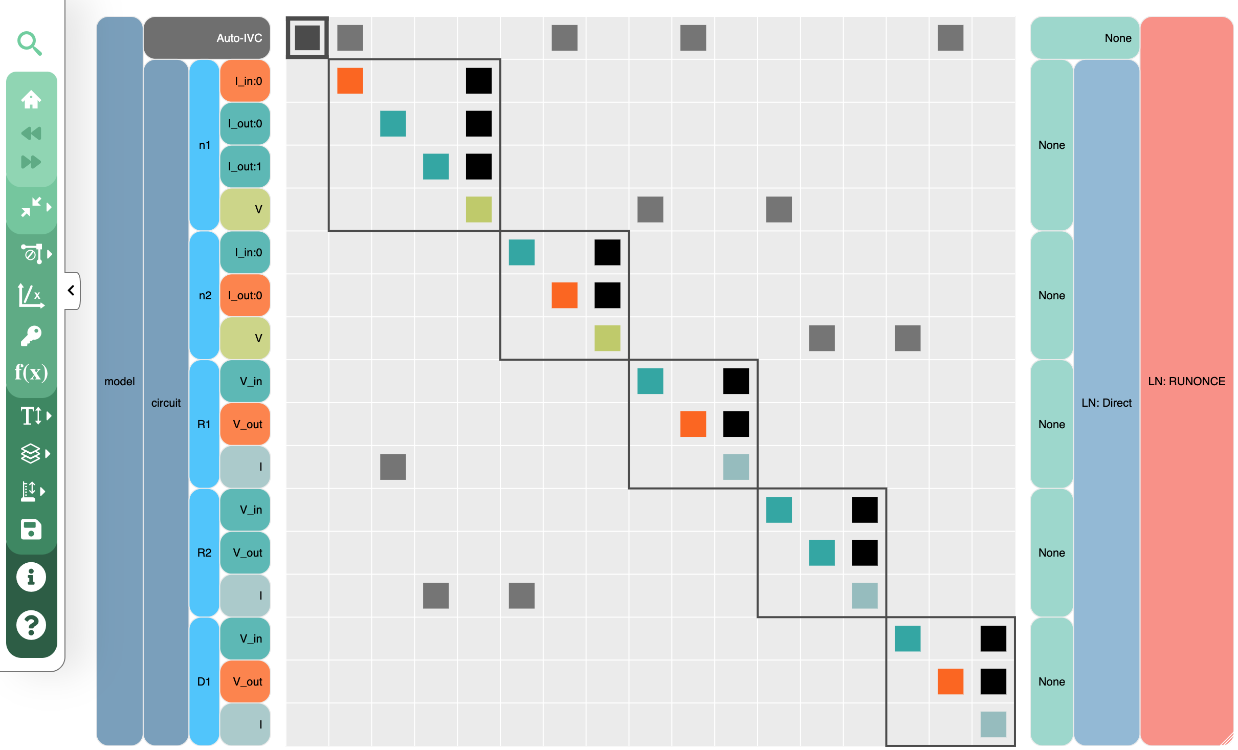
Here is the N2 diagram that is generated from this model. There are three parts to the N2 diagram. The model hierarchy is on the left, the connection matrix is displayed in the center, and the solver hierarchy is shown on the right.

Model Hierarchy#

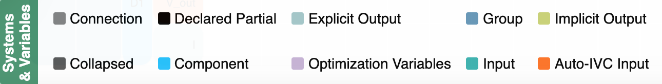
The model hierarchy is on the left side of the diagram. It is a mix of Systems and variables, both inputs and outputs.

The top System, the root of the model, is on the left and the subsystem hierarchy is displayed to its right.

The colors indicate the type of item in the hierarchy. To see what the colors represent, an optional legend can be displayed using the button. Here is the part of the legend that explains the colors of the model hierarchy.

systems_and_variables_legend

You can click in the model hierarchy to zoom into, and also collapse and expand sections of the hierarchy. Left clicking on a subsystem zooms the hierarchy display to just that subsystem in the hierarchy. Right clicking on a subsystem collapses all of the hierarchy to the right of it.

Buttons on the toolbar, which are explained in the Toolbar section, also can be used to control what is displayed in the hierarchy.

Connection Matrix#

The matrix in the middle of the diagram shows what items in the model are connected.

The color of an item on a diagonal cell matches the color of the rightmost element in the model hierarchy. The colors for the off-diagonal items, which indicate connections, are always black.

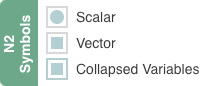
The symbol of an item in the connection matrix indicates whether the variable is a scalar, vector, or collapsed variable.

connection_matrix_legend

Boxes, with thin black line borders, outline items in the matrix to show the grouping of the variables of the lowest level Systems.

When you hover over a connection in the matrix, arrows are drawn to indicate connections. The behavior is different depending on whether you hover over a diagonal or an off-diagonal cell.

When hovering over a diagonal item, the explicit connections to/from that variable are displayed. Salmon colored arrows indicate that element is the target of the connection. A green arrow indicates it is the source.

When hovering over an off-diagonal, the behavior differs depending on whether the cell is in the lower or upper triangular part of the diagram.

In the lower triangular, the marked cells represent upstream (in the sense of execution order of the components) connections. All the connections involved in that cycle are drawn to indicate which systems and components are involved in the convergence loop. Downstream connection arrows are green and upstream connections are salmon colored.

In the upper triangular, the marked cells represent downstream connections. The salmon colored arrow that is drawn shows that connection.

Clicking in the matrix on a connection or diagonal, lets you pin connection arrows so that they don’t disappear when you hover away from the cell. You can clear these connections arrows by using the Hide all connection arrow button in the toolbar.

Solver Hierarchy#

Each System in a model can potentially have a linear and nonlinear solver associated with it. On the right side of the N2 diagram, the hierarchy of the solvers is shown. This time the hierarchy goes from right to left with the root of the model on the right.

There are three states of the solver hierarchy display. Use these buttons to switch between them. Hiding the solver hierarchy creates more space for the rest of the N2 display.

Button	Title	Description
	Show linear solvers	Show linear solvers in solver hierarchy
	Show non-linear solvers	Show non-linear solvers in solver hierarchy
	Hide Solvers	Hide the solver hierarchy

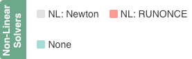
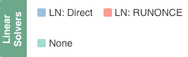
The colors indicate the type of solver. The colors are shown in the legend. The section of the legend showing the colors of the solver types changes depending on which are displayed in the solver structure. Here is what the section of the legend looks like for both linear and non-linear solvers.

Non-Linear Solver Legend	Linear Solver Legend

Note

When a System has a Newton non-linear solver and the solve_subsystems option is set to True for that solver, the Solver hierarchy box for that System has the text NL: Newton (sub_solve).

As in the model hierarchy, you can also do zooming, collapsing, and expanding in the Solver hierarchy using left and right mouse clicks.

Toolbar#

The toolbar to the left of the N2 diagram provides many useful capabilities. Explanations for all the buttons is below. Tooltips are also provided for all the buttons as you hover over them.

View Control#

The model hierarchy display has the notion of a view. The view is defined by the node in the hierarchy that is visible in the diagram. Initially, it is the root of the model but if you click on a subsystem, then only the part of the hierarchy beginning at that subsystem is shown.

You can change the view and zoom into a System by left clicking on it. Other parts of the hierarchy are no longer visible.

The diagram keeps track of the view history and then lets you go back and forth through the history similar to undo and redo in apps.

Button	Title	Description
	Return to root	View entire model starting from root
	Back	Move back in view history
	Forward	Move forward in view history

Collapsing and Expanding the System Hierarchy#

The next set of buttons lets you control the collapsing and expanding of elements in the System hierarchy. The first four buttons are revealed as a fly-out menu as you hover over this button, forward .

Button	Title	Description
	Collapse variables in view only	Collapse only the variables in the current view
	Expand variables in view only	Expand only the variables in the current view
	Collapse all variables	Collapse all the variables in the entire model
	Expand all variables	Expand all the variables in the entire model
	Collapse depth	Set the number of hierarchy levels shown in the view

Connections Arrow Visibility#

The connections visibility is controlled using the buttons that appear when hovering over the button.

Button	Title	Description
	Hide all connection arrows	Hide all pinned connection arrows.
	Show all connections in view	Show all connections in view and pin them.

Remaining Toolbar Buttons#

The buttons in the remaining part of the toolbar offer a variety of other options:

Button	Title	Description
	Show legend / Hide legend	Show the legend explaining the colors and icons in the diagram
	Show opt vars / Hide opt vars	Show the optimization variables in the diagram
	Font Size	Set the font size for the text in the diagram
	Set collapse depth	Set how many levels are shown in the System hierarchy on the left
	Model Height	Set the height of the diagram in pixels
	Save SVG	Save the current view of the diagram to an SVG file
	Show / Hide Node Info	Toggle info box that is displayed on hover
	Help	Bring up the help window

Show Legend#

If you click on the legend button show_legend , you will see the legend appear below the N2 diagram. The Legend window can then be dragged to a location of the user’s choice.

legend

Here are explanations of the sections in the legend:

The System & Variables section shows the colors for the different items in the model hierarchy.
The N2 Symbols section shows the icons used to indicate the type of connection in the connection matrix. The shape of the icon in the matrix shows whether the connection is between scalars, vectors, or groups. The color of the icon is based on the color associated with the variable of that type as shown in the System & Variables part of the legend.
The Solvers section shows the colors used for the different solvers on the right side of the N2. Either the Linear or Nonlinear solvers are shown depending on the state of the Toggle Solver Names button.

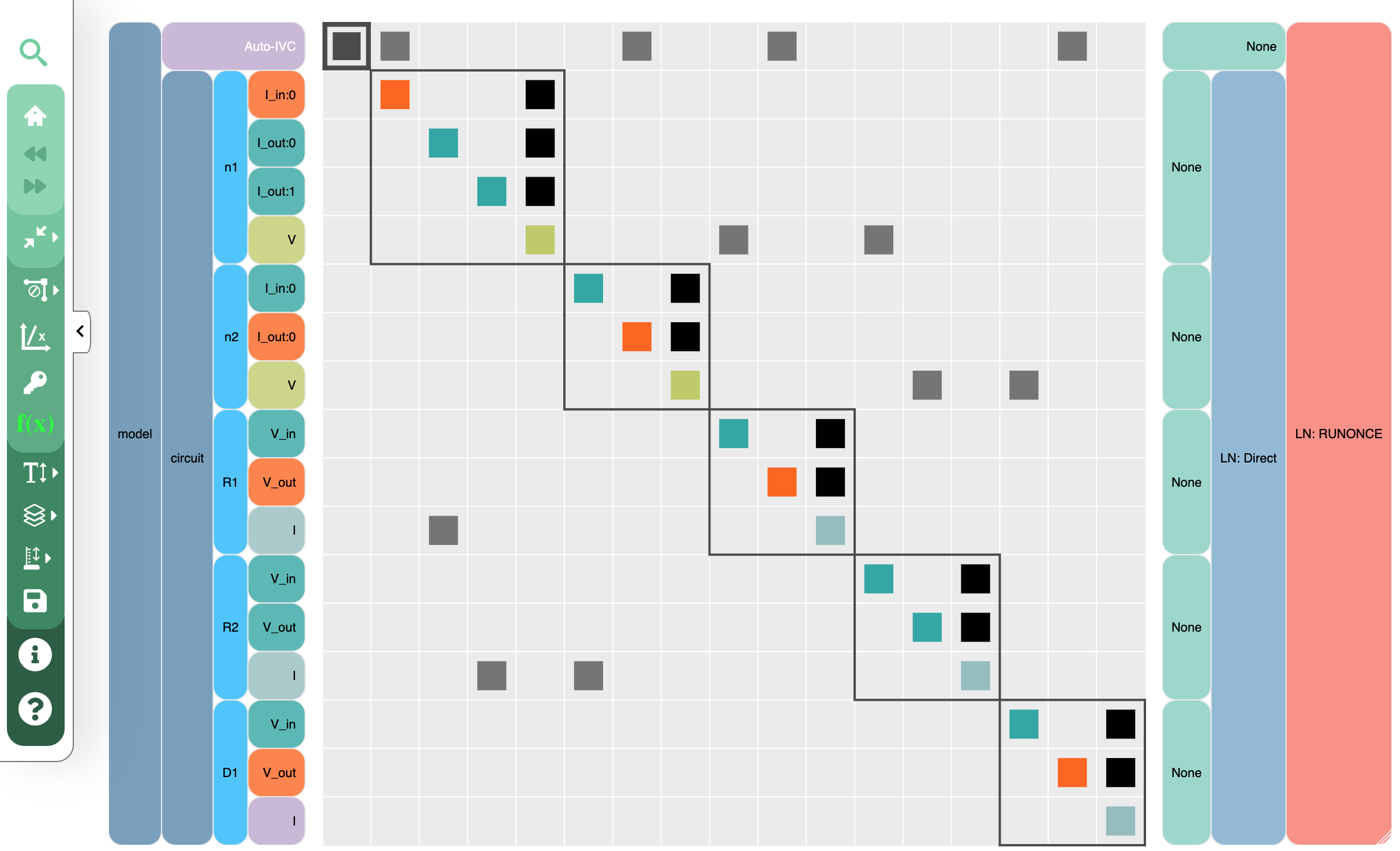
Show/Hide Optimization Variables#

Selecting this button model_opt_button allows you to see your model’s design variables, constraints, and objectives which are highlighted in purple. If your optimization variable is an Auto IVC, the Auto IVC cell will be highlighted as well which can be seen below.

Hidden	Shown

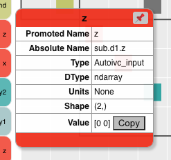
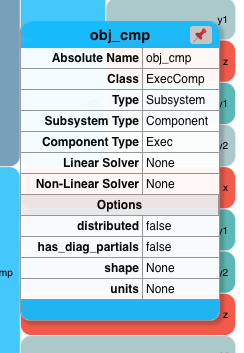
Show Node Info#

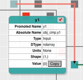
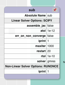
The Show Node Info button |show_node_info|, brings up a small window that displays information about the item the cursor is hovering over. Here are some examples of what the user can see when hovering over variables, Systems, connection matrix cells, and Solvers.

Variable	System	Connection	Solver

Search bar#

The search bar below the Toolbar lets you search for variables in the model. This can be very useful when working with very large models.

When you enter a variable name into the search box and click the search button or hit the Enter key, the N2 diagram will redraw such that it collapses and shows only variables that were searched for.

A search could find multiple instances of variables with the same name. For example, in the diagram above, a search for V_in would find R1.V_in, R2.V_in, and D1.V_in.

To return to a view that is not filtered by the variable search, clear the search box and hit the Enter key or the Search button.

Show external connections#

When you zoom into a System, it is useful to see external connections into that System from other Systems that are no longer visible as a result of zooming. In that situation, the N2 diagram indicates external connections with dashed line arrows. For example:

external_connection

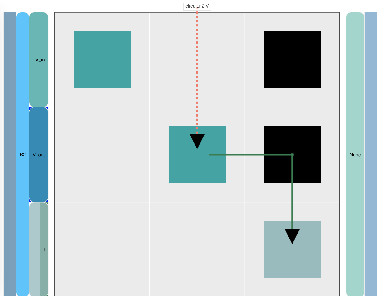
The dashed line arrow shows that R2.V_out variable is connected to circuit.n2.V even though that variable is no longer visible in the diagram.