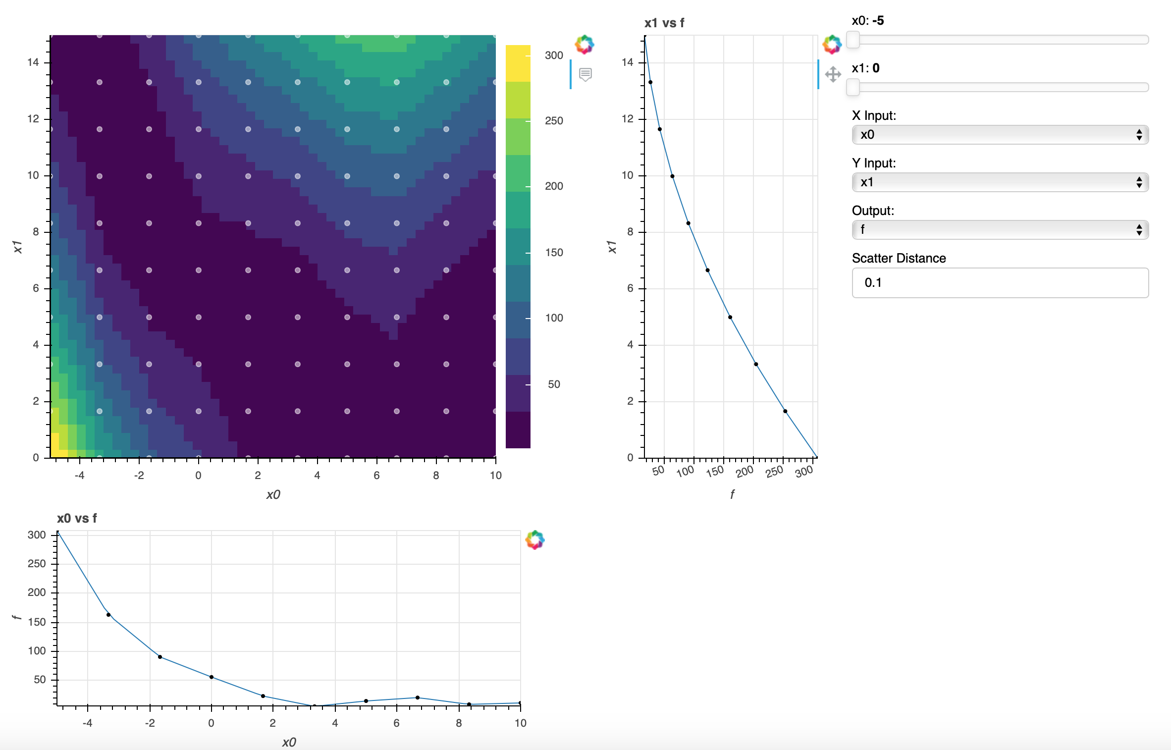
Metamodel Visualization#
When evaluating meta models, it can be useful to determine their fit of the training data, graphically.
OpenMDAO has a visualization package to view the training data and meta models generated from it.
This page explains how to use view_mm in the command line.
The metamodel viewer allows a user the ability of reducing a high dimensional input space down to three dimensions to enable the user to determine the fit of a meta model to the given training data.
Running the Visualizer#

Note
This tool is accessible through the OpenMDAO command line tools which can be found om-command.
Running openmdao view_mm structured_meta_model_example.py will open the metamodel generated
from the script in the browser and generate a metamodel viewer like the one below. The user can adjust
sliders to make slices in the graph, change X and Y inputs, and change the scatter distance value to
fine tune the distance a point can be from the model line.
To recreate the viewer above, copy the first script given below and paste it into a file named structured_meta_model_example.py. Next, run openmdao view_mm structured_meta_model_example.py in the command line.
Structured MetaModel Example Script#
import numpy as np
import openmdao.api as om

num_train = 10

x0_min, x0_max = -5.0, 10.0
x1_min, x1_max = 0.0, 15.0
train_x0 = np.linspace(x0_min, x0_max, num_train)
train_x1 = np.linspace(x1_min, x1_max, num_train)
t_data = np.array([[308.12909601, 253.61567418, 204.6578079, 161.25549718, 123.40874201, 91.1175424,   64.38189835,  43.20180985,  27.5772769,   17.50829952],
                [162.89542418, 123.20470795,  89.06954726,  60.48994214,  37.46589257, 19.99739855,   8.08446009,   1.72707719,   0.92524984,   5.67897804,],
                [ 90.2866907,   63.02637433,  41.32161352,  25.17240826,  14.57875856, 9.54066442,  10.05812583,  16.13114279,  27.75971531,  44.94384339,],
                [ 55.60211264,  38.37989042,  26.71322375,  20.60211264,  20.04655709, 25.04655709,  35.60211264,  51.71322375,  73.37989042, 100.60211264],
                [ 22.81724065,  13.24080685,   9.2199286,   10.75460591,  17.84483877, 30.49062719, 48.69197117,  72.4488707,  101.76132579, 136.62933643],
                [  5.11168719,   0.78873608,   2.02134053,   8.80950054,  21.1532161, 39.05248721,  62.50731389,  91.51769611, 126.0836339,  166.20512723],
                [ 14.3413983,   12.87962416,  16.97340558,  26.62274256,  41.82763509, 62.58808317,  88.90408682, 120.77564601, 158.20276077, 201.18543108],
                [ 20.18431209,  19.1914092,   23.75406186,  33.87227009,  49.54603386, 70.77535319,  97.56022808, 129.90065853, 167.79664453, 211.24818608],
                [  8.48953212,   5.57319475,   8.21241294,  16.40718668,  30.15751598, 49.46340083,  74.32484124, 104.74183721, 140.71438873, 182.2424958 ],
                [ 10.96088904,   3.72881146,   2.05228945,   5.93132298,  15.36591208, 30.35605673,  50.90175693,  77.00301269, 108.65982401, 145.87219088]])

prob = om.Problem()
mm = prob.model.add_subsystem('mm', om.MetaModelStructuredComp(method='slinear'),
                            promotes=['x0', 'x1'])
mm.add_input('x0', 0.0, train_x0)
mm.add_input('x1', 0.0, train_x1)
mm.add_output('f', 0.0, t_data)

prob.setup()
prob.final_setup()
Unstructured MetaModel Example Script#
To view this example metamodel, copy the following script into a file named unstructured_meta_model_example.py and then run openmdao view_mm unstructured_meta_model_example.py in the command line.
from math import pi

# Model
interp = om.MetaModelUnStructuredComp()

# Training Data
x_train1 = np.random.uniform(0, pi, 100)
x_train2 = np.random.uniform(0, pi, 100)
x_train3 = np.random.uniform(0, pi, 100)
y = np.sin(x_train1 * x_train2 * x_train3)

# Inputs
interp.add_input('input_1', 0., training_data=x_train1)
interp.add_input('input_2', 0., training_data=x_train2)
interp.add_input('input_3', 0., training_data=x_train3)

# Outputs
interp.add_output('output_1', 0., training_data=y)

# Surrogate Model
interp.options['default_surrogate'] = om.KrigingSurrogate()

prob = om.Problem()
prob.model.add_subsystem('interp', interp)
prob.setup()
prob.final_setup()
Note
OpenMDAO supports structured and unstructured metamodels. Please refer to the documentation for a more in depth overview of what Unstructured and Structured metamodels are.
Multiple Meta Models in Script#
If your model has multiple metamodels, you can specify which of them you want to visualize. For example, in this code there are two metamodels.
class CosMetaModel(om.MetaModelUnStructuredComp):
    def setup(self):
        # Training Data
        x_train = np.linspace(0, 10, 20)
        y_train = np.linspace(0, 20, 20)

        # Inputs
        self.add_input('x', 0., training_data=x_train)
        self.add_input('y', 0., training_data=y_train)

        # Outputs
        self.add_output('cos_x', 0., training_data=np.cos(x_train + y_train))

        # Surrogate Model
        self.options['default_surrogate'] = om.ResponseSurface()


class SinMetaModel(om.MetaModelUnStructuredComp):
    def setup(self):
        # Training Data
        x_train = np.linspace(0, 10, 20)
        y_train = np.linspace(0, 20, 20)

        # Inputs
        self.add_input('x', 0., training_data=x_train)
        self.add_input('y', 0., training_data=y_train)

        # Outputs
        self.add_output('sin_x', 0., training_data=np.sin(x_train + y_train))

        # Surrogate Model
        self.options['default_surrogate'] = om.ResponseSurface()


# define model with two metamodel components
model = om.Group()
cos_mm = model.add_subsystem('cos_mm', CosMetaModel())
sin_mm = model.add_subsystem('sin_mm', SinMetaModel())

# setup a problem using our dual metamodel model
prob = om.Problem(model)
prob.setup()
prob.final_setup()
To visualize only the first one, you would use the command:
openmdao view_mm -m cos_mm multiple_metamodels.py
Command Line Interface#
The command, openmdao view_mm requires a file path, the name of the meta model which you want to visualize if there is more than one, and optionally a port number:
openmdao view_mm -h
usage: openmdao view_mm [-h] [-m PATHNAME] [-r RESOLUTION] [-p PORT_NUMBER]
                        [--no_browser]
                        file

positional arguments:
  file                  Python file containing the model.

options:
  -h, --help            show this help message and exit
  -m, --metamodel_pathname PATHNAME
                        pathname of the metamodel component.
  -r, --resolution RESOLUTION
                        Number of points to create contour grid
  -p, --port_number PORT_NUMBER
                        Port number to open viewer
  --no_browser          Bokeh server will start server without browser
Note
When using Bash on Windows you are required to set –no_browser option to start the server and then open an internet browser and copy/paste the path to viewer. Bash on Windows does not allow the terminal to access your browser to open the viewer.
