Using the Case Viewer#
The CaseViewer is a tool for interactive viewing of recorded cases data in Jupyter notebooks. This is currently an experimental feature of OpenMDAO but it’s useful enough in its current state that we’ve included it in the package.
Example: Queen Dido’s Problem#
Queen Dido’s problem is an optimization problem that is also a legend about the founding of Carthage. Supposedly Queen Dido was allowed all the land she could enclose within the hide of an ox. Cutting the hide into very thin strips provided her with a long, but finite, length of “fencing.” What arrangement of this fencing provides the greatest possible enclosed area?
If we assume a straight edge along one side of the fence (such as a riverbank or shoreline), how should the fencing be arranged to capture the greatest possible area?
The following component takes the distance of the river bank, \(L\), as well as the distance of the “fence posts” from the riverbank, \(y\), and computes the enclosed area and the perimeter.
import openmdao.api as om
import numpy as np
class Fence(om.ExplicitComponent):

    def initialize(self):
        self.options.declare('n', types=int, default=50, desc='number of fenceposts')

    def setup(self):
        n = self.options['n']
        self.add_input('L', val=10.0, units='m')
        self.add_input('y', val=np.zeros(n), units='m')

        self.add_output('perimeter', val=0.0, units='m')
        self.add_output('area', val=0.0, units='m**2')
        self.add_output('x', val=np.linspace(0, 100, n), units='m')

        self.declare_partials(of='*', wrt='*', method='cs')

    def compute(self, inputs, outputs):
        n = self.options['n']
        L = inputs['L']
        y = inputs['y']

        x = np.linspace(0, L, n)

        dx = x[1:] - x[:-1]
        dy = y[1:] - y[:-1]

        mean_y = 0.5 * (y[1:] + y[:-1])

        outputs['perimeter'] = np.sum(np.sqrt(dx**2+dy**2))
        outputs['area'] = np.sum(dx * mean_y)
        outputs['x'] = x
The optimization problem is to arrange these fence posts such that the perimeter \(p\) does not exceed some value while maximizing the enclosed area \(A\).
In addition, the first and last fenceposts should be placed along the river’s edge.
<Figure size 1200x600 with 3 Axes>
Solving the Optimization Problem and Recording the Driver Iterations#
In the following code, we set up the optimization problem to find the location of 20 fence posts which maximize area while limiting perimeter to \(300\) meters. A recorder is added to the driver that records the design variables, constraints, and objectives.
N = 20
p = om.Problem()

p.model.add_subsystem('fence', Fence(n=N))

p.model.add_design_var('fence.L', lower=1)
p.model.add_design_var('fence.y', lower=0, indices=om.slicer[1:-1])
p.model.add_constraint('fence.perimeter', equals=100 * np.pi, ref=100 * np.pi)
p.model.add_objective('fence.area', ref=-1000.0)

p.driver = om.pyOptSparseDriver(optimizer='SLSQP')

p.driver.add_recorder(om.SqliteRecorder('driver_cases.db'))
p.driver.recording_options['includes'] = ['*']
p.driver.recording_options['record_desvars'] = True
p.driver.recording_options['record_constraints'] = True
p.driver.recording_options['record_objectives'] = True

p.setup(force_alloc_complex=True)

p.set_val('fence.y', val=np.zeros(N))

p.run_driver();
Optimization Problem -- Optimization using pyOpt_sparse
================================================================================
    Objective Function: _objfunc

    Solution:
--------------------------------------------------------------------------------
    Total Time:                    0.2689
       User Objective Time :       0.0974
       User Sensitivity Time :     0.1422
       Interface Time :            0.0217
       Opt Solver Time:            0.0076
    Calls to Objective Function :      35
    Calls to Sens Function :           32


   Objectives
      Index  Name                  Value
          0  fence.area    -8.218499E-01

   Variables (c - continuous, i - integer, d - discrete)
      Index  Name         Type      Lower Bound            Value      Upper Bound     Status
          0  fence.L_0       c     1.000000E+00     1.069717E+01     1.000000E+30
          1  fence.y_0       c     0.000000E+00     2.185646E+00     1.000000E+30
          2  fence.y_1       c     0.000000E+00     3.139145E+00     1.000000E+30
          3  fence.y_2       c     0.000000E+00     3.783755E+00     1.000000E+30
          4  fence.y_3       c     0.000000E+00     4.258652E+00     1.000000E+30
          5  fence.y_4       c     0.000000E+00     4.617809E+00     1.000000E+30
          6  fence.y_5       c     0.000000E+00     4.885983E+00     1.000000E+30
          7  fence.y_6       c     0.000000E+00     5.077885E+00     1.000000E+30
          8  fence.y_7       c     0.000000E+00     5.202154E+00     1.000000E+30
          9  fence.y_8       c     0.000000E+00     5.263328E+00     1.000000E+30
         10  fence.y_9       c     0.000000E+00     5.263328E+00     1.000000E+30
         11  fence.y_10      c     0.000000E+00     5.202154E+00     1.000000E+30
         12  fence.y_11      c     0.000000E+00     5.077885E+00     1.000000E+30
         13  fence.y_12      c     0.000000E+00     4.885983E+00     1.000000E+30
         14  fence.y_13      c     0.000000E+00     4.617809E+00     1.000000E+30
         15  fence.y_14      c     0.000000E+00     4.258652E+00     1.000000E+30
         16  fence.y_15      c     0.000000E+00     3.783755E+00     1.000000E+30
         17  fence.y_16      c     0.000000E+00     3.139145E+00     1.000000E+30
         18  fence.y_17      c     0.000000E+00     2.185646E+00     1.000000E+30

   Constraints (i - inequality, e - equality)
      Index  Name            Type          Lower           Value           Upper    Status  Lagrange Multiplier (N/A)
          0  fence.perimeter    e   1.000000E+00    1.000000E+00    1.000000E+00              9.00000E+100


   Exit Status
      Inform  Description
           0  Optimization terminated successfully.
--------------------------------------------------------------------------------
Invoking the CaseViewer#
In the following line we invoke the CaseViewer. It will not be displayed in the static documentation here, but executing this notebook in Jupyter will provide a GUI like that shown in the figure below.
om.CaseViewer(p.get_outputs_dir() / 'driver_cases.db');
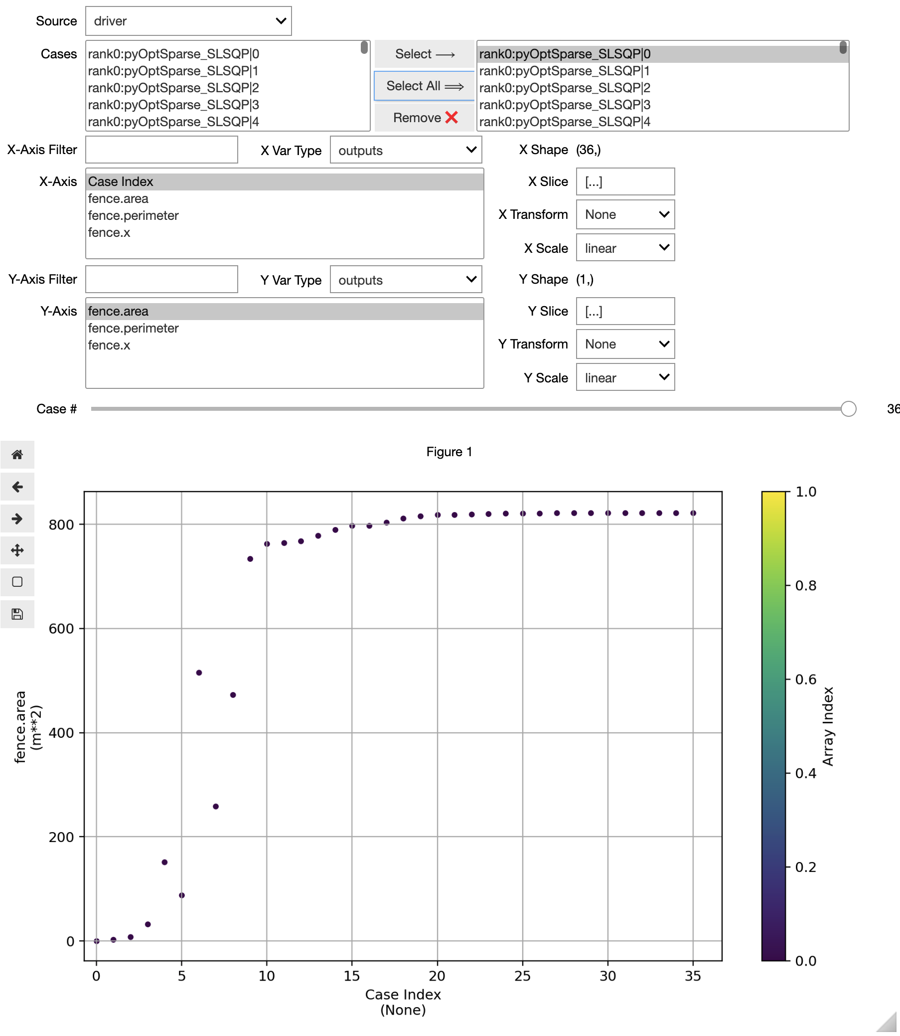
Plotting a scalar vs. the case index#
To see how the value of a variable evolves over the iteration history, use Case Index as the X-Axis variable.
For instance, to see how the area (the objective function) changes over iterations, choose outputs -> fence.area as the Y-Axis variable.
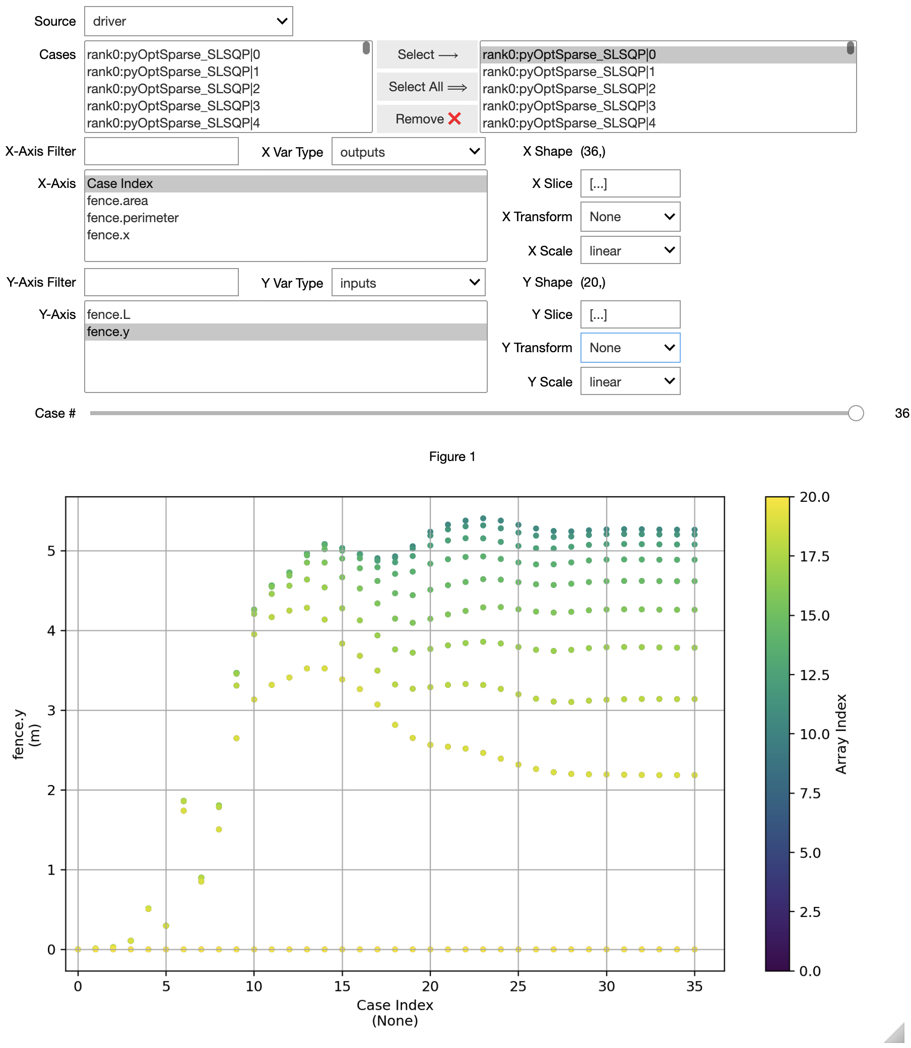
Plotting an array vs. the case index#
When an array-valued variable is plotted against the Case Index, each value in the array is plotted at the X-Axis value corresponding to each case. The color of each point represents its index in the array, with warmer colors being higher indices.
For instance, to see how the values of fence.y at each iteration, choose inputs -> fence.y as the Y-Axis variable.
If this type of plot is too noisy for your data, you can use the Y Transform options to retrieve things like the maximum value in the array, the minimum value in the array, or the norm of the array.
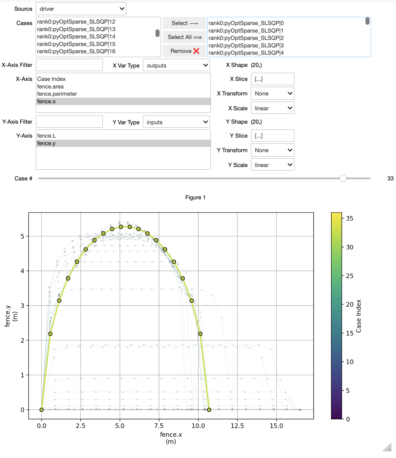
Plotting one array vs. another#
Sometimes it’s useful to visualize the evolution of a solution as the plot of one array-shaped variable vs. another.
In our case, the shape of the fence is represented by plotting outputs -> fence.x on the X-Axis and inputs -> fence.y on the Y-Axis.
When plotting arrays, the X-Axis is required to be viewable as a flattened array.
The Y-Axis variable must have the same number of points as the X-Axis variable in its first dimension.
In our use-case here, fence.x and fence.y have the same shape.
If they did not, then the slice text boxes could be used to reshape the variable in the appropriate way.
The default value, [...], plots the entire array.
When plotting one array vs. another, the CaseViewer will connect the points in each case using a line, and color that line based on the index of the case in the selected cases box at the top of the GUI. Scrolling the slider will highlight a particular case.
Current limitations of the CaseViewer#
CaseViewer is currently limited to one instance per notebook. Instantiating more than one will cause the plotting interface to fail.