Determining Variable Shapes at Runtime

It’s sometimes useful to create a component where the shapes of its inputs and/or outputs are determined by their connections. This allows us to create components representing general purpose vector or matrix operations such as norms, summations, integrators, etc., that size themselves appropriately based on the model that they’re added to.

Turning on dynamic shape computation is straightforward. You just specify shape_by_conn, copy_shape and/or compute_shape in your add_input or add_output calls when you add variables to your component.

Setting shape_by_conn=True when adding an input or output variable will allow the shape of that variable to be determined at runtime based on the variable that connects to it.

Setting copy_shape=<var_name>, where <var_name> is the local name of another variable in your component, will take the shape of the variable specified in <var_name> and use that shape for the variable you’re adding.

Setting compute_shape=<func>, where <func> is a function taking a dict arg that maps variable names to shapes and returning the computed shape, will set the shape of the variable you’re adding as a function of the other variables in the same component of the opposite io type. For example, setting compute_shape for an output z on a component with inputs x and y, would cause the supplied function to be called with a dict of the form {x: , y: }, so the computed shape of z could be a function of the shapes of x and y.

Note that shape_by_conn can be specified for outputs as well as for inputs, as can copy_shape and compute_shape. This means that shape information can propagate through the model in either forward or reverse. If you specify both shape_by_conn and either copy_shape or compute_shape for your component’s dynamically shaped variables, it will allow their shapes to be resolved whether known shapes have been defined upstream or downstream of your component in the model.

For example, the following component with input x and output y can have its shapes set by known shapes that are either upstream or downstream. Note that this component also has sparse partials, diagonal in this case, and those are specified within the setup_partials method which is called after all shapes have been computed. It uses the _get_var_meta method to get the size of its variables in order to determine the size of the partials.

import openmdao.api as om


class DynPartialsComp(om.ExplicitComponent):
    def setup(self):
        self.add_input('x', shape_by_conn=True, copy_shape='y')
        self.add_output('y', shape_by_conn=True, copy_shape='x')

    def setup_partials(self):
        size = self._get_var_meta('x', 'size')
        self.mat = np.eye(size) * 3.
        rng = np.arange(size)
        self.declare_partials('y', 'x', rows=rng, cols=rng, val=3.0)

    def compute(self, inputs, outputs):
        outputs['y'] = self.mat.dot(inputs['x'])

The following example demonstrates the flow of shape information in the forward direction, where the IndepVarComp has a known size, and the DynPartialsComp and the ExecComp are sized dynamically.

import numpy as np

p = om.Problem()
p.model.add_subsystem('indeps', om.IndepVarComp('x', val=np.ones(5)))
p.model.add_subsystem('comp', DynPartialsComp())
p.model.add_subsystem('sink', om.ExecComp('y=x',
                                          x={'shape_by_conn': True, 'copy_shape': 'y'},
                                          y={'shape_by_conn': True, 'copy_shape': 'x'}))
p.model.connect('indeps.x', 'comp.x')
p.model.connect('comp.y', 'sink.x')
p.setup()
p.run_model()
J = p.compute_totals(of=['sink.y'], wrt=['indeps.x'])
print(J['sink.y', 'indeps.x'])

[[ 3. -0. -0. -0. -0.]
 [-0.  3. -0. -0. -0.]
 [-0. -0.  3. -0. -0.]
 [-0. -0. -0.  3. -0.]
 [-0. -0. -0. -0.  3.]]

And the following shows shape information flowing in reverse, from the known shape of sink.x to the unknown shape of the output comp.y, then to the input comp.x, then on to the connected auto-IndepVarComp output.

import numpy as np

p = om.Problem()
p.model.add_subsystem('comp', DynPartialsComp())
p.model.add_subsystem('sink', om.ExecComp('y=x', shape=5))
p.model.connect('comp.y', 'sink.x')
p.setup()
p.run_model()
J = p.compute_totals(of=['sink.y'], wrt=['comp.x'])
print(J['sink.y', 'comp.x'])

[[ 3. -0. -0. -0. -0.]
 [-0.  3. -0. -0. -0.]
 [-0. -0.  3. -0. -0.]
 [-0. -0. -0.  3. -0.]
 [-0. -0. -0. -0.  3.]]

Finally, an example use of compute_shape is shown below. We have a dynamically shaped component that multiplies two matrices, so the output O shape is determined by the shapes of both inputs, M and N. In this case we use a lambda function to compute the output shape.

import numpy as np

class DynComputeComp(om.ExplicitComponent):
    def setup(self):
        self.add_input('M', shape_by_conn=True)
        self.add_input('N', shape_by_conn=True)

        # use a lambda function to compute the output shape based on the input shapes
        self.add_output('O', compute_shape=lambda shapes: (shapes['M'][0], shapes['N'][1]))

    def compute(self, inputs, outputs):
        outputs['O'] = inputs['M'] @ inputs['N']

p = om.Problem()
indeps = p.model.add_subsystem('indeps', om.IndepVarComp())
indeps.add_output('M', val=np.ones((3, 2)))
indeps.add_output('N', val=np.ones((2, 5)))
p.model.add_subsystem('comp', DynComputeComp())
p.model.connect('indeps.M', 'comp.M')
p.model.connect('indeps.N', 'comp.N')
p.setup()
p.run_model()
print('input shapes:', p['indeps.M'].shape, 'and', p['indeps.N'].shape)
print('output shape:', p['comp.O'].shape)

input shapes: (3, 2) and (2, 5)
output shape: (3, 5)

Residuals, like partials, have shapes which depend upon the shapes of the inputs of the component. The add_residual method for implicit components is typically used in the setup method, but in situations where the inputs are dynamically shaped, this information is not known at this time.

For this reason, implicit components support a setup_residuals method. This method is called in final_setup after the shapes of all inputs and outputs is known.

For instance, the InputResidsComp in OpenMDAO adds a corresponding residual for each input. Since these inputs may use dynamic sizing, we cannot assume to know their shapes during setup. As a result, the setup_residuals method is used in InputResidsComp to add the residuals once their shapes are known:

from openmdao.utils.notebook_utils import get_code
from myst_nb import glue
glue("input_resids_comp_src", get_code("openmdao.components.input_resids_comp.InputResidsComp"), display=False)

Debugging

Sometimes, when the shapes of some variables are unresolvable, it can be difficult to understand why. There is an OpenMDAO command line tool, openmdao view_dyn_shapes, that can be used to show a graph of the dynamically shaped variables and any statically shaped variables that connect directly to them. Each node in the graph is a variable, and each edge is a connection between that variable and another. Note that this connection does not have to be a connection in the normal OpenMDAO sense. It could be a connection internal to a component created by declaring a copy_shape in the metadata of one variable that refers to another variable.

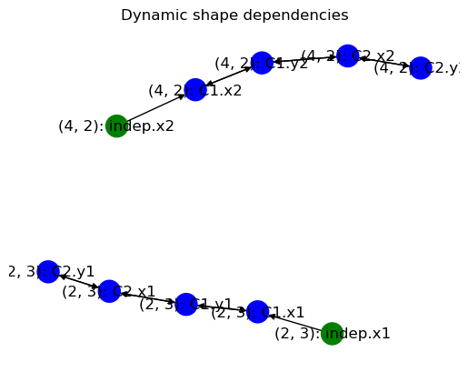
The nodes in the graph are colored to make it easier to locate static/dynamic/unresolved variable shapes. Statically shaped variables are colored green, dynamically shaped variables that have been resolved are colored blue, and any variables with unresolved shapes are colored red. Each node is labeled with the shape of the variable, if known, or a ‘?’ if unknown, followed by the absolute pathname of the variable in the model.

The plot is somewhat crude and the node labels sometimes overlap, but it’s possible to zoom in to part of the graph to make it more readable using the button that looks like a magnifying glass.

Below is an example plot for a simple model with three components and no unresolved shapes.

Connecting Non-Distributed and Distributed Variables

Dynamically shaped connections between distributed outputs and non-distributed inputs are not allowed because OpenMDAO assumes data will be transferred locally when computing variable shapes. Since non-distributed variables must be identical in size and value on all ranks where they exist, the distributed output would have to also be identical in size and value on all ranks. If that is the case, then the output should just be non-distributed as well.

Dynamically shaped connections between non-distributed outputs and distributed inputs are currently allowed, though their use is not recommended. Such connections require that all src_indices in all ranks of the distributed input are identical.