Timing Systems under MPI#
There is a way to view timings for methods called on specific group and component instances in an OpenMDAO model when running under MPI. It displays how that model spends its time across MPI processes.
The simplest way to use it is via the command line using the openmdao timing command. For example:
mpirun -n <nprocs> openmdao timing <your_python_script_here>
This will collect the timing data and generate a text report that could look something like this:
  Problem: main   method: _solve_nonlinear

    Parallel group: traj.phases (ncalls = 3)

    System                 Rank      Avg Time     Min Time     Max_time   Total Time
    ------                 ----      --------     --------     --------   ----------
    groundroll                0        0.0047       0.0047       0.0048       0.0141
    rotation                  0        0.0047       0.0047       0.0047       0.0141
    ascent                    0        0.0084       0.0083       0.0085       0.0252
    accel                     0        0.0042       0.0042       0.0042       0.0127
    climb1                    0        0.0281       0.0065       0.0713       0.0843
    climb2                    1       21.7054       1.0189      57.5102      65.1161
    climb2                    2       21.6475       1.0189      57.3367      64.9426
    climb2                    3       21.7052       1.0188      57.5101      65.1156

    Parallel group: traj2.phases (ncalls = 3)

    System                 Rank      Avg Time     Min Time     Max_time   Total Time
    ------                 ----      --------     --------     --------   ----------
    desc1                     0        0.0479       0.0041       0.1357       0.1438
    desc1                     1        0.0481       0.0041       0.1362       0.1444
    desc2                     2        0.0381       0.0035       0.1072       0.1143
    desc2                     3        0.0381       0.0035       0.1073       0.1144

    Parallel group: traj.phases.climb2.rhs_all.prop.eng.env_pts (ncalls = 3)

    System                 Rank      Avg Time     Min Time     Max_time   Total Time
    ------                 ----      --------     --------     --------   ----------
    node_2                    1        4.7018       0.2548      13.0702      14.1055
    node_5                    1        4.6113       0.2532      12.5447      13.8338
    node_8                    1        5.4608       0.2538      15.3201      16.3824
    node_11                   1        5.8348       0.2525      13.3362      17.5044
    node_1                    2        4.8227       0.2534      13.3842      14.4680
    node_4                    2        5.1912       0.2526      14.4703      15.5737
    node_7                    2        5.4818       0.2524      15.3875      16.4454
    node_10                   2        4.3591       0.2530      12.2027      13.0773
    node_0                    3        5.0172       0.2501      14.1460      15.0515
    node_3                    3        5.1350       0.2493      14.3048      15.4050
    node_6                    3        5.3238       0.2487      14.9546      15.9715
    node_9                    3        4.9638       0.2502      14.0088      14.8914
There will be a section of the report for each ParallelGroup in the model, and each section has a header containing the name of the ParallelGroup method being called and the number of times that method was called. Each section contains a line for each subsystem in that ParallelGroup for each MPI rank where that subsystem is active. Each of those lines will show the subsystem name, the MPI rank, and the average, minimum, maximum, and total execution time for that subsystem on that rank.
In the table shown above, the model was run using 4 processes, and we can see that in the
traj.phases parallel group, there is an uneven distribution of average execution times among its
6 subsystems. The traj.phases.climb2 subsystem takes far longer to execute (approximately
21 seconds vs. a fraction of a second) than any of the other subsystems in traj.phases, so it makes
sense that it is being given more processes (3) than the others. In fact, all of the other subsystems
share a single process. The relative execution times are so different in this case that it would
probably decrease the overall execution time if all of the subsystems in traj.phases were run
on all 4 processes. This is certainly true if we assume that the execution time of climb2 will
decrease in a somewhat linear fashion as we let it run on more processes. If that’s the case then
we could estimate the sequential execution time of climb2 to be around 65 seconds, so, assuming
linear speedup it’s execution time would decrease to around 16 seconds, which is about 5 seconds
faster than the case shown in the table. The sum of execution times of all of the other subsystems
combined is only about 1/20th of a second, so duplicating all of them on all processes will cost us
far less than we saved by running climb2 on 4 processes instead of 3.
If the openmdao timing command is run with a -v option of ‘browser’ (see arguments below), then
an interactive table view will be shown in the browser and might look something like this:
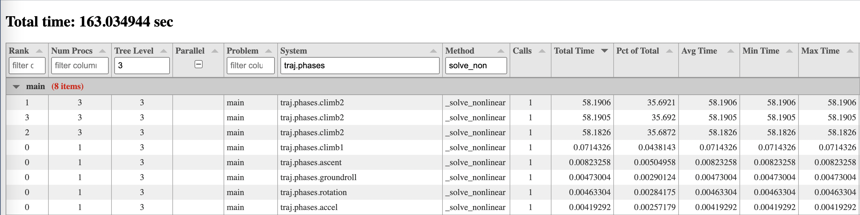
There is a row in the table for each method specified for each group or component instance in the model, on each MPI rank. The default method is _solve_nonlinear, which gives a good view of how the timing of nonlinear
execution breaks down for different parts of the system tree. _solve_nonlinear is a framework method
that calls compute for explicit components and apply_nonlinear for implicit ones. If you’re more
interested in timing of derivative computations, you could use the -f or --function args
(see arg descriptions below) to add _linearize, which calls compute_partials for explicit components
and linearize for implicit ones, and/or _apply_linear, which calls compute_jacvec_product
for explicit components or apply_linear for implicit ones. The reason to add the framework
methods _solve_nonlinear, _linearize, and _apply_linear instead of the component level ones
like compute, etc. is that the framework methods are called on both groups and components
and so provide a clearer way to view timing contributions of subsystems to their parent ParallelGroup
whether those subsystems happen to be components or groups.
There are columns in the table for mpi rank, number of procs, level in the system tree, whether a system is the child of a parallel group or not, problem name, system path, method name, number of calls, total time, percent of total time, average time, min time, and max time. If the case was not run under more than one MPI process, then the columns for mpi rank, number of procs, parallel columns will not be shown. All columns are sortable, and most are filterable except those containing floating point numbers.
Documentation of options for all commands described here can be obtained by running the command followed by the -h option. For example:
openmdao timing -h
usage: openmdao timing [-h] [-o OUTFILE] [-f FUNCS] [-v VIEW] [--use_context] file

positional arguments:
  file                  Python file containing the model, or pickle file containing previously recorded timing
                        data.

optional arguments:
  -h, --help            show this help message and exit
  -o OUTFILE            Name of output file where timing data will be stored. By default it goes to
                        "timings.pkl".
  -f FUNCS, --func FUNCS
                        Time a specified function. Can be applied multiple times to specify multiple functions.
                        Default methods are ['_apply_linear', '_solve_nonlinear'].
  -v VIEW, --view VIEW  View of the output. Default view is 'text', which shows timing for each direct child of a
                        parallel group across all ranks. Other options are ['browser', 'dump', 'none'].
  --use_context         If set, timing will only be active within a timing_context.
If you don’t like the default set of methods, you can specify your own using the -f or --funct options.
This option can be applied multiple times to specify multiple functions.
The -v and --view options default to “text”, showing a table like the one above. You can also
choose “browser” which will display an interactive table in a browser, “dump” which will give you
essentially an ascii dump of the table data, or “none” which generates no output other than a pickle
file, typically “timings.pkl” that contains the timing data and can be used for later viewing.
The --use_context option is for occasions when you only want to time a certain portion of your script.
In that case, you can wrap the code of interest in a timing_context context manager as shown below.
from openmdao.visualization.timing_viewer.timer import timing_context

# do some stuff that I don't want to time...

with timing_context():
    # do stuff I want to time
    pass

# do some other stuff that I don't want to time...
Warning
If the use_context option is set, timing will not occur anywhere outside of timing_context, so be careful not to use that option on a script that doesn’t use a timing_context, because in that case, no timing will be done.
Warning
If you don’t specify use_context but your script does contain a timing_context, then that timing_context will be ignored and timing info will be collected for the entire script anyway.
After your script is finished running, you should see a new file called timings.pkl in your current directory. This is a pickle file containing all of the timing data. If you specified a view option of “browser”, you’ll also see a file called timing_report.html which can be opened in a browser to view the interactive timings table discussed earlier.
Warning
If your script exits with a nonzero exit code, the timing data will not be saved to a file.