SplineComp#
SplineComp allows you to represent a larger dimensional variable with a smaller dimensional variable by using an interpolation algorithm. This is useful for reducing the size of an optimization problem by decreasing the number of design variables it solves. The spatial distribution of the points, in both the original and interpolated spaces is typically uniform but other distributions can be used.
Note
OpenMDAO contains two components that perform interpolation: SplineComp and MetaModelStructuredComp.
While they provide access to mostly the same algorithms, their usage is subtly different.
The fundamental differences between them are as follows:
MetaModelStructuredComp is used when you have a set of known data values y on a structured grid x and want to interpolate a new y value at a new x location that lies inside the grid. In this case, you generally start with a known set of fixed “training” values and their locations.
SplineComp is used when you want to create a smooth curve with a large number of points, but you
want to control the shape of the curve with a small number of control points. The x locations of
the interpolated points (and where applicable, the control points) are fixed and known, but the
y values at the control points vary as the curve shape is modified by an upstream connection.
MetaModelStructuredComp can be used for multi-dimensional design spaces, whereas SplineComp is restricted to one dimension.
The following methods are available by setting the ‘method’ option:
Method |
Order |
Description |
|---|---|---|
slinear |
1 |
Basic linear interpolation |
lagrange2 |
2 |
Second order Lagrange polynomial |
lagrange3 |
3 |
Third order Lagrange polynomial |
akima |
3 |
Interpolation using Akima splines |
cubic |
3 |
Cubic spline, with continuity of derivatives between segments |
bsplines |
var. |
BSplines, default order is 4. |
scipy_slinear |
1 |
Scipy linear interpolation. Same as slinear, though slower |
scipy_cubic |
3 |
Scipy cubic interpolation. More accurate than cubic, but slower |
scipy_quintic |
5 |
Scipy quintic interpolation. Most accurate, but slowest |
SplineComp Options#
| Option | Default | Acceptable Values | Acceptable Types | Description |
|---|---|---|---|---|
| always_opt | False | [True, False] | ['bool'] | If True, force nonlinear operations on this component to be included in the optimization loop even if this component is not relevant to the design variables and responses. |
| default_shape | (1,) | N/A | ['tuple'] | Default shape for variables that do not set val to a non-scalar value or set shape, shape_by_conn, copy_shape, or compute_shape. Default is (1,). |
| derivs_method | N/A | ['jax', 'cs', 'fd', None] | N/A | The method to use for computing derivatives |
| distributed | False | [True, False] | ['bool'] | If True, set all variables in this component as distributed across multiple processes |
| interp_options | {} | N/A | ['dict'] | Dict contains the name and value of options specific to the chosen interpolation method. |
| method | akima | ['slinear', 'lagrange2', 'lagrange3', 'cubic', 'akima', 'bsplines', 'scipy_cubic', 'scipy_slinear', 'scipy_quintic'] | N/A | Spline interpolation method to use for all outputs. |
| num_cp | N/A | N/A | ['int'] | Number of spline control points. Optional alternative to x_cp_val. Required for bsplines. If None, num_cp will be a linspace from 0 to 1. |
| run_root_only | False | [True, False] | ['bool'] | If True, call compute, compute_partials, linearize, apply_linear, apply_nonlinear, solve_linear, solve_nonlinear, and compute_jacvec_product only on rank 0 and broadcast the results to the other ranks. |
| use_jit | True | [True, False] | ['bool'] | If True, attempt to use jit on compute_primal, assuming jax or some other AD package capable of jitting is active. |
| vec_size | 1 | N/A | ['int'] | Number of points to evaluate at once. |
| x_cp_val | N/A | N/A | ['list', 'ndarray'] | List/array of x control point values, must be monotonically increasing. Optional alternative to num_cp. Not applicable for bsplines. |
| x_interp_val | **Required** | N/A | ['list', 'ndarray'] | List/array of x interpolated point values. |
SplineComp Constructor#
The call signature for the SplineComp constructor is:
- SplineComp.__init__(**kwargs)[source]
Initialize all attributes.
SplineComp Basic Example#
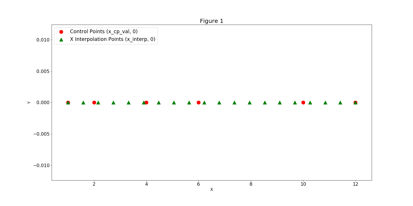
In our example, we have a pre-generated curve that is described by a series of values y_cp at a
sequence of locations x_cp, and we would like to interpolate new values at multiple locations
between these points. We call these new fixed locations at which to interpolate: x. When we
instantiate a SplineComp, we specify these x_cp and x locations as numpy arrays and pass
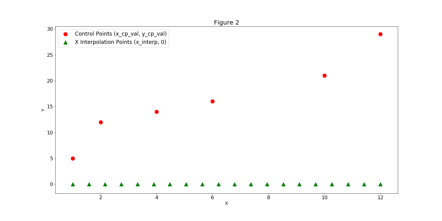
them in as constructor keyword arguments. (Figure 1). Next we’ll add our y_cp data in by
calling the add_spline method and passing the y_cp values in as the keyword argument y_cp_val (Figure 2).
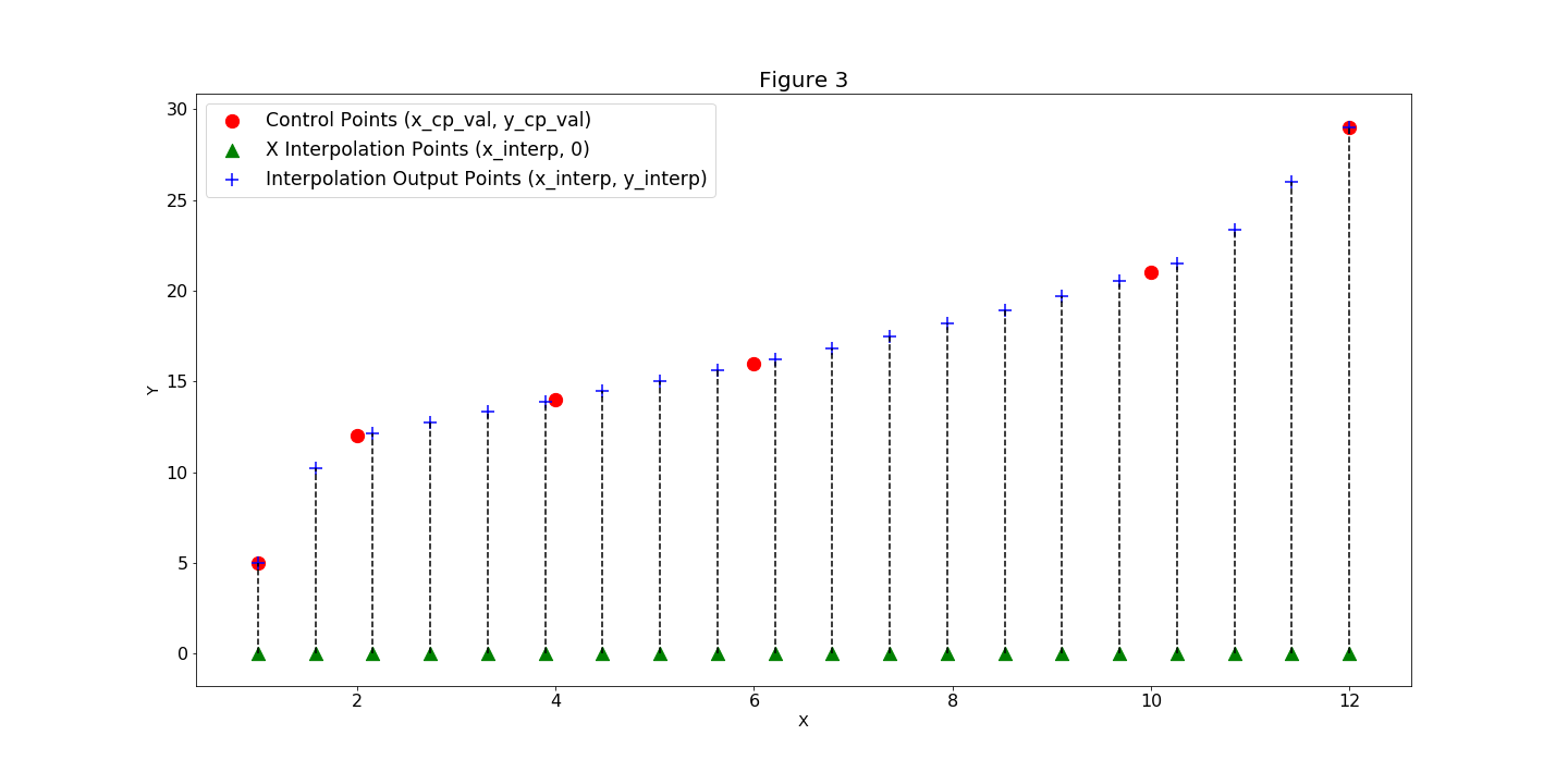
SplineComp computes and outputs the y_interp values (Figure 3).
import numpy as np
import openmdao.api as om

xcp = np.array([1.0, 2.0, 4.0, 6.0, 10.0, 12.0])
ycp = np.array([5.0, 12.0, 14.0, 16.0, 21.0, 29.0])
n = 50
x = np.linspace(1.0, 12.0, n)

prob = om.Problem()

akima_option = {'delta_x': 0.1}
comp = om.SplineComp(method='akima', x_cp_val=xcp, x_interp_val=x,
                     interp_options=akima_option)

prob.model.add_subsystem('akima1', comp)

comp.add_spline(y_cp_name='ycp', y_interp_name='y_val', y_cp_val=ycp)

prob.setup(force_alloc_complex=True)
prob.run_model()

print(prob.get_val('akima1.y_val'))
[[ 5.          7.20902005  9.21276849 10.81097162 11.80335574 12.1278001
  12.35869145 12.58588536 12.81022332 13.03254681 13.25369732 13.47451633
  13.69584534 13.91852582 14.14281484 14.36710105 14.59128625 14.81544619
  15.03965664 15.26399335 15.48853209 15.7133486  15.93851866 16.16573502
  16.39927111 16.63928669 16.8857123  17.1384785  17.39751585 17.66275489
  17.93412619 18.21156029 18.49498776 18.78433915 19.07954501 19.38053589
  19.68724235 19.99959495 20.31752423 20.64096076 20.96983509 21.37579297
  21.94811407 22.66809748 23.51629844 24.47327219 25.51957398 26.63575905
  27.80238264 29.        ]]
SplineComp Multiple Splines#
SplineComp supports multiple splines on a fixed x_interp grid. Below is an example of how a user can
setup two splines on a fixed grid. To do this the user needs to pass in names to give to the component
input and output. The initial values for y_cp can also be specified here.
x_cp = np.array([1.0, 2.0, 4.0, 6.0, 10.0, 12.0])
y_cp = np.array([5.0, 12.0, 14.0, 16.0, 21.0, 29.0])
y_cp2 = np.array([1.0, 5.0, 7.0, 8.0, 13.0, 16.0])
n = 50
x = np.linspace(1.0, 12.0, n)

prob = om.Problem()

comp = om.SplineComp(method='akima', x_cp_val=x_cp, x_interp_val=x)
prob.model.add_subsystem('akima1', comp)

comp.add_spline(y_cp_name='ycp1', y_interp_name='y_val1', y_cp_val=y_cp)
comp.add_spline(y_cp_name='ycp2', y_interp_name='y_val2', y_cp_val=y_cp2)

prob.setup(force_alloc_complex=True)
prob.run_model()
Specifying Options for ‘akima’#
When you are using the ‘akima’ method, there are two akima-specific options that can be passed in to the
SplineComp constructor. The ‘delta_x’ option is used to define the radius of the smoothing interval
that is used in the absolute values functions in the akima calculation in order to make their
derivatives continuous. This is set to zero by default, which effectively turns off the smoothing.
The ‘eps’ option is used to define the value that triggers a division-by-zero
safeguard; its default value is 1e-30.
x_cp = np.array([1.0, 2.0, 4.0, 6.0, 10.0, 12.0])
y_cp = np.array([5.0, 12.0, 14.0, 16.0, 21.0, 29.0])

n = 50
x = np.linspace(1.0, 12.0, n)

prob = om.Problem()
model = prob.model

# Set options specific to akima
akima_option = {'delta_x': 0.1, 'eps': 1e-30}

comp = om.SplineComp(method='akima', x_cp_val=x_cp, x_interp_val=x,
                     interp_options=akima_option)

prob.model.add_subsystem('atmosphere', comp)

comp.add_spline(y_cp_name='alt_cp', y_interp_name='alt', y_cp_val=y_cp, y_units='kft')

prob.setup(force_alloc_complex=True)
prob.run_model()
Specifying Options for ‘bsplines’#
When you use the ‘bsplines’ method, you can specify the bspline order by defining ‘order’ in an otherwise empty dictionary and passing it in as ‘interp_options’.
In addition, when using ‘bsplines’, you cannot specify the ‘x_cp’ locations because the bspline algorithm places them at fixed locations. The starting and ending control points are at the starting and ending interpolation points respectively. You can specify the number of control points using the ‘num_cp’ argument. You can also change the mapping of the control points by specifying the location of the first and/or last control point. This is done by defining ‘x_cp_start’ and/or ‘x_cp_end’ in the’interp_options’ dictionary mentioned above.
prob = om.Problem()
model = prob.model

n_cp = 80
n_point = 160

t = np.linspace(0, 3.0*np.pi, n_cp)
tt = np.linspace(0, 3.0*np.pi, n_point)
x = np.sin(t)

# Set options specific to bsplines
bspline_options = {'order': 3}

comp = om.SplineComp(method='bsplines', x_interp_val=tt, num_cp=n_cp,
                    interp_options=bspline_options)

prob.model.add_subsystem('interp', comp, promotes_inputs=[('h_cp', 'x')])

comp.add_spline(y_cp_name='h_cp', y_interp_name='h', y_cp_val=x, y_units=None)

prob.setup(force_alloc_complex=True)
prob.set_val('x', x)
prob.run_model()
SplineComp Interpolation Distribution#
The cell_centered function takes the number of cells, and the start and end values, and returns a
vector of points that lie at the center of those cells. The ‘node_centered’ function reproduces the
functionality of numpy’s linspace. Finally, the sine_distribution function creates a sinusoidal
distribution, in which points are clustered towards the ends. A ‘phase’ argument is also included,
and a phase of pi/2.0 clusters the points in the center with fewer points on the ends.
Note
We have included three different distribution functions for users to replicate functionality that used to be built-in to the individual akima and bsplines components.
- openmdao.utils.spline_distributions.sine_distribution(num_points, start=0.0, end=1.0, phase=3.141592653589793)[source]
Sine distribution of control points.
- Parameters:
- num_pointsint
Number of points to predict at.
- startint or float
Minimum value to interpolate at.
- endint or float
Maximum value to interpolate at.
- phasefloat
Phase of the sine wave.
- Returns:
- ndarray
Values to interpolate at.
- openmdao.utils.spline_distributions.cell_centered(num_cells, start=0.0, end=1.0)[source]
Cell centered distribution of control points.
- Parameters:
- num_cellsint
Number of cells.
- startint or float
Minimum value to interpolate at.
- endint or float
Maximum value to interpolate at.
- Returns:
- ndarray
Values to interpolate at.
- openmdao.utils.spline_distributions.node_centered(num_points, start=0.0, end=1.0)[source]
Distribute control points.
- Parameters:
- num_pointsint
Number of points to predict.
- startint or float
Minimum value to interpolate at.
- endint or float
Maximum value to interpolate at.
- Returns:
- ndarray
Values to interpolate at.
Below is an example of sine_distribution
x_cp = np.linspace(0., 1., 6)
y_cp = np.array([5.0, 12.0, 14.0, 16.0, 21.0, 29.0])
n = 20
x = om.sine_distribution(20, start=0, end=1, phase=np.pi)

prob = om.Problem()

comp = om.SplineComp(method='akima', x_cp_val=x_cp, x_interp_val=x)
prob.model.add_subsystem('akima1', comp)

comp.add_spline(y_cp_name='ycp', y_interp_name='y_val', y_cp_val=y_cp)

prob.setup(force_alloc_complex=True)
prob.run_model()

print(prob.get_val('akima1.y_val'))
[[ 5.          5.32381994  6.28062691  7.79410646  9.64169506 11.35166363
  12.26525921 12.99152288 13.77257256 14.58710327 15.41289673 16.28341046
  17.96032258 20.14140712 22.31181718 24.40891577 26.27368825 27.74068235
  28.67782484 29.        ]]
Standalone Interface for Spline Evaluation#
The underlying interpolation algorithms can be used standalone (i.e., outside of the SplineComp) through the
InterpND class. This can be useful for inclusion in another component. The following example shows how to
create and evaluate a standalone Akima spline:
from openmdao.components.interp_util.interp import InterpND

xcp = np.array([1.0, 2.0, 4.0, 6.0, 10.0, 12.0])
ycp = np.array([5.0, 12.0, 14.0, 16.0, 21.0, 29.0])
n = 50
x = np.linspace(1.0, 12.0, n)

interp = InterpND(method='akima', points=xcp, x_interp=x, delta_x=0.1)
y = interp.evaluate_spline(ycp)

print(y)
[ 5.          7.20902005  9.21276849 10.81097162 11.80335574 12.1278001
 12.35869145 12.58588536 12.81022332 13.03254681 13.25369732 13.47451633
 13.69584534 13.91852582 14.14281484 14.36710105 14.59128625 14.81544619
 15.03965664 15.26399335 15.48853209 15.7133486  15.93851866 16.16573502
 16.39927111 16.63928669 16.8857123  17.1384785  17.39751585 17.66275489
 17.93412619 18.21156029 18.49498776 18.78433915 19.07954501 19.38053589
 19.68724235 19.99959495 20.31752423 20.64096076 20.96983509 21.37579297
 21.94811407 22.66809748 23.51629844 24.47327219 25.51957398 26.63575905
 27.80238264 29.        ]
Similiarly, the following example shows how to create a bspline:
from openmdao.components.interp_util.interp import InterpND

xcp = np.array([1.0, 2.0, 4.0, 6.0, 10.0, 12.0])
ycp = np.array([5.0, 12.0, 14.0, 16.0, 21.0, 29.0])
n = 50
x = np.linspace(1.0, 12.0, n)

interp = InterpND(method='bsplines', num_cp=6, x_interp=x)

y = interp.evaluate_spline(ycp)

print(y)
[ 5.          6.21958113  7.31225085  8.28604153  9.14898554  9.90911525
 10.57446302 11.15306122 11.65294223 12.08213839 12.4486821  12.7606057
 13.02594157 13.25272208 13.44897959 13.62274647 13.7820551  13.93461483
 14.08438023 14.23288341 14.38161608 14.53206997 14.68573681 14.84410832
 15.00867623 15.18093226 15.36236815 15.5544756  15.75874636 15.97667213
 16.20974466 16.45945567 16.72729687 17.01478976 17.32524076 17.66472303
 18.03954772 18.45602598 18.92046894 19.43918775 20.01849357 20.66469753
 21.38411079 22.18304448 23.06780976 24.04471776 25.12007964 26.30020655
 27.59140962 29.        ]
You can also compute the derivative of the interpolated output with respect to the control point values by setting the “compute_derivate” argument to True:
from openmdao.components.interp_util.interp import InterpND

xcp = np.array([1.0, 2.0, 4.0, 6.0, 10.0, 12.0])
ycp = np.array([5.0, 12.0, 14.0, 16.0, 21.0, 29.0])
n = 5
x = np.linspace(1.0, 12.0, n)

interp = InterpND(method='akima', points=xcp, x_interp=x, delta_x=0.1)
y, dy_dycp = interp.evaluate_spline(ycp, compute_derivative=True)

print(dy_dycp)
[[ 1.00000000e+00  0.00000000e+00  0.00000000e+00  0.00000000e+00
   0.00000000e+00  0.00000000e+00]
 [-1.86761492e-06  3.31278014e-02  1.05874907e+00 -9.18750000e-02
   0.00000000e+00  0.00000000e+00]
 [ 0.00000000e+00  0.00000000e+00 -2.10964627e-01  1.19119941e+00
   2.02602810e-02 -4.95062934e-04]
 [ 0.00000000e+00  0.00000000e+00 -2.64126732e-01  5.82784977e-01
   6.83151998e-01 -1.81024253e-03]
 [ 0.00000000e+00  0.00000000e+00  0.00000000e+00  0.00000000e+00
   0.00000000e+00  1.00000000e+00]]