MetaModelSemiStructuredComp

MetaModelSemiStructuredComp#

Semi-structued training data occurs frequently in engineering applications like performance maps for turbine engine performance, propeller performance, aerodyanmic drag, etc. For example, a simple semi-structured grid could be a mostly structured grid, but with a few data points missing on one area of the grid. Another more general kind of semi-structured grid is a set of data where the first dimension is regular, but the other dimensions are irregular. An example of this is the figure below, where the ‘x’ dimension is regular, and the data points fall on distinct values, but the ‘y’ dimension is not regular.

semi_example

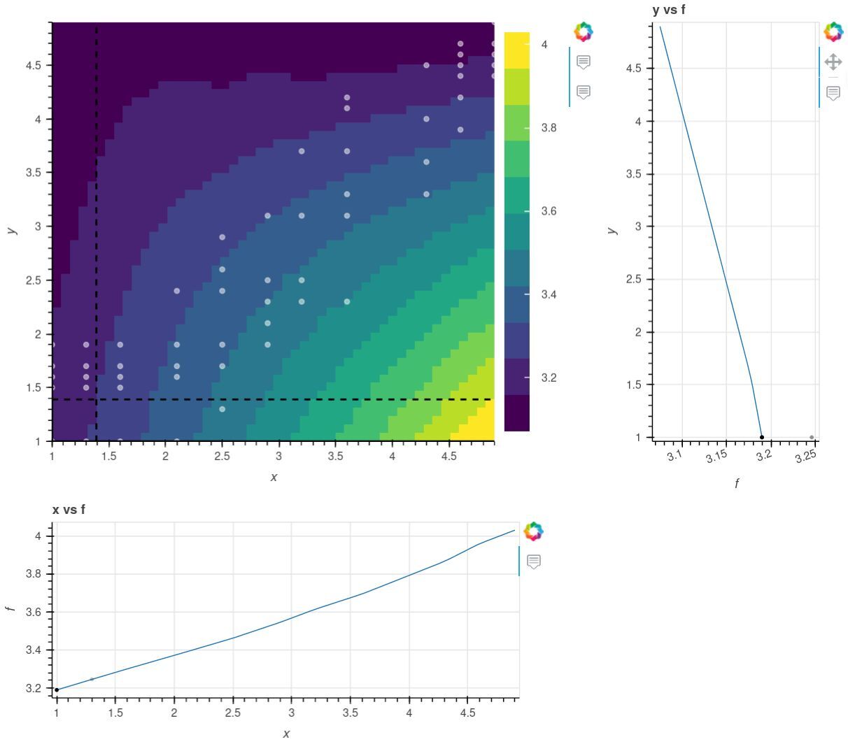
The MetaModelStructured cannot be used if any points are missing, or if any dimension is not regular. You could use MetaModelUnStructured for this data, but you would lose the performance and flexibility you can gain from exploiting the semi structured nature of the data.

MetaModelSemiStructuredComp handles semi-structured data by treating every “column” of data beyond the first dimension independently. In the figure above, it doesn’t matter that two adjacent columns have different points, as the interpolation in ‘y’ happens independently in each column before those values are subsequently interpolated in ‘x’.

The following interpolation methods are supported in MetaModelSemiStructuredComp:

Method	Order	Description
slinear	1	Basic linear interpolation
lagrange2	2	Second order Lagrange polynomial
lagrange3	3	Third order Lagrange polynomial
akima	3	Interpolation using Akima splines

Note that MetaModelSemiStructuredComp only accepts scalar inputs and outputs. If you have a multivariable function, each input variable needs its own named OpenMDAO input.

For multi-dimensional data, fits are computed on a separable per-axis basis. A single interpolation method is used for all dimensions, so the minimum table dimension must be high enough to use the chosen interpolate. Further, the minimum dimension will potentially be driven by the sparsest area of your data, so care should be taken to choose the smallest regular dimension as the first dimension.

Extrapolation is supported, and is enabled by default. Given the more sparse nature of semi-structured data, we expect that extrapolation will occur more often. When evaluating a point, if any of the requested values falls beyond the first or last point in a row, you are extrapolating. There is always a risk when extrapolating, so it is important to be careful. Extrapolation can be disabled via the extrapolate option (see below).

MetaModelSemiStructuredComp Options#

Option	Default	Acceptable Values	Acceptable Types	Description
always_opt	False	[True, False]	['bool']	If True, force nonlinear operations on this component to be included in the optimization loop even if this component is not relevant to the design variables and responses.
derivs_method	N/A	['jax', 'cs', 'fd', None]	N/A	The method to use for computing derivatives
distributed	False	[True, False]	['bool']	If True, set all variables in this component as distributed across multiple processes
extrapolate	True	[True, False]	['bool']	Sets whether extrapolation should be performed when an input is out of bounds.
method	slinear	['slinear', 'lagrange2', 'lagrange3', 'akima']	N/A	Spline interpolation method to use for all outputs.
run_root_only	False	[True, False]	['bool']	If True, call compute, compute_partials, linearize, apply_linear, apply_nonlinear, and compute_jacvec_product only on rank 0 and broadcast the results to the other ranks.
training_data_gradients	False	[True, False]	['bool']	When True, compute gradients with respect to training data values.
use_jit	True	[True, False]	['bool']	If True, attempt to use jit on compute_primal, assuming jax or some other AD package is active.
vec_size	1	N/A	['int']	Number of points to evaluate at once.

MetaModelSemiStructuredComp Constructor#

The call signature for the MetaModelSemiStructuredComp constructor is:

MetaModelSemiStructuredComp.__init__(**kwargs)[source]

Initialize all attributes.

MetaModelSemiStructuredComp Examples#

A simple quick-start example is fitting a 2-dimensional data set that has been evaluated on a small selection of semi structured points:

import numpy as np

data_x = np.array([
0,
0,
0,
0,
0,

3,
3,
3,
3,
3,

6,
6,
6,
6,
6,

1,
1,
1,
1,
1,

5,
5,
5,
5,
5,
5,

9,
9,
9,
9,
9,

2,
2,
2,
2,

6,
6,
6,
6,
6,
6,

3,
3,
3,
3,

6,
6,
6,
6,
6,
6,

9,
9,
9,
9,
9,
])

data_y = np.array([
0,
5,
6,
7,
9,

0,
5,
6,
7,
9,

0,
5,
6,
7,
9,

0,
6,
7,
9,
4,

3,
7,
9,
4,
6,
9,

9,
1,
3,
5,
1,

3,
5,
1,
7,

3,
1,
3,
7,
1,
2,

3,
6,
0,
5,

9,
2,
4,
5,
6,
7,

4,
5,
6,
7,
9,
])

data_values = 3.0 + np.sin(data_x*0.2) * np.cos(data_y*0.3)

Notice that the table input data is expressed as flat ndarrays (or lists). They should be sorted in ascending coordinate order starting with the lowest n-tuple. The table output values are also in a flat array that corresponds to the input arrays.

import openmdao.api as om

prob = om.Problem()
model = prob.model

interp = om.MetaModelSemiStructuredComp(method='lagrange2')

# The order that the inputs are added matters. The first table dimension is 'x'.
interp.add_input('x', data_x)
interp.add_input('y', data_y)

interp.add_output('f', training_data=data_values)

# Including a second output to show that multiple outputs are supported.
# All outputs use the same input grid but use different values at each point.
interp.add_output('g', training_data=2.0 * data_values)
        
model.add_subsystem('interp', interp)

prob.setup()

prob.set_val('interp.x', np.array([3.1]))
prob.set_val('interp.y', np.array([2.75]))

prob.run_model()

print(prob.get_val('interp.f'), prob.get_val('interp.g'))

[3.39415716] [6.78831431]

You can also predict multiple independent output points by setting the vec_size argument to be equal to the number of points you want to predict. Here, we set it to 3 and predict 3 points with MetaModelSemiStructuredComp:

prob = om.Problem()
model = prob.model

interp = om.MetaModelSemiStructuredComp(method='lagrange2', vec_size=3)

# The order that the inputs are added matters. The first table dimension is 'x'.
interp.add_input('x', data_x)
interp.add_input('y', data_y)

interp.add_output('f', training_data=data_values)

model.add_subsystem('interp', interp)

prob.setup()

prob.set_val('interp.x', np.array([3.1, 4.7, 5.1]))
prob.set_val('interp.y', np.array([2.75, 3.9, 4.2]))

prob.run_model()

print(prob.get_val('interp.f'))

[3.39415716 3.31511313 3.2608656 ]

Finally, it is possible to compute gradients with respect to the given output training data. These gradients are not computed by default, but can be enabled by setting the option training_data_gradients to True. When this is done, for each output that is added to the component, a corresponding input is added to the component with the same name but with an _train suffix. This allows you to connect in the training data as an input array, if desired.

The following simple example shows the preceding model with training inputs enabled.

prob = om.Problem()
model = prob.model

interp = om.MetaModelSemiStructuredComp(method='lagrange2', training_data_gradients=True)
interp.add_input('x', data_x)
interp.add_input('y', data_y)

# Initialize all trable values to zero.
interp.add_output('f', training_data=np.zeros(len(data_x)))

model.add_subsystem('interp', interp)

prob.setup(force_alloc_complex=True)

prob.set_val('interp.x', np.array([3.1]))
prob.set_val('interp.y', np.array([2.75]))

# The table values come from somewhere in OpenMDAO, in this case, from the indepvarcomp output.
# They could also come from an upstream component if you connect the input to another source.
prob.set_val('interp.f_train', data_values)

prob.run_model()

print(prob.get_val('interp.f'))

[3.39415716]

Standalone Interface for Table Interpolation#

The underlying interpolation algorithms can be used standalone (i.e., outside of the MetaModelSemiStructuredComp) through the InterpNDSemi class. This can be useful for inclusion in another component. The following component shows how to perform interpolation on the a much simpler table than before. We only have 2 points at x=1.0, so we can only choose ‘slinear’.

from openmdao.components.interp_util.interp_semi import InterpNDSemi

# Simple grid with one point missing.
x = [1.0, 1.0, 2.0, 2.0, 2.0]
y = [1.0, 2.0, 1.0, 2.0, 3.0]
values = [1.0, 2.5, 1.5, 4.0, 4.5]

grid = np.array([x, y]).T
print(grid)

# We only have 2 points at x=1.0, so 'slinear' is the only one we can use.
interp = InterpNDSemi(grid, values, method='slinear')

x = np.array([1.5, 1.5])
f, df_dx = interp.interpolate(x, compute_derivative=True)

print('value', f)
print('derivative', df_dx)

[[1. 1.]
 [1. 2.]
 [2. 1.]
 [2. 2.]
 [2. 3.]]
value [2.25]
derivative [[1. 2.]]