The Brachistochrone with Externally-Sourced Controls#
Things you’ll learn through this example
How to provide trajectory control values from an external source.
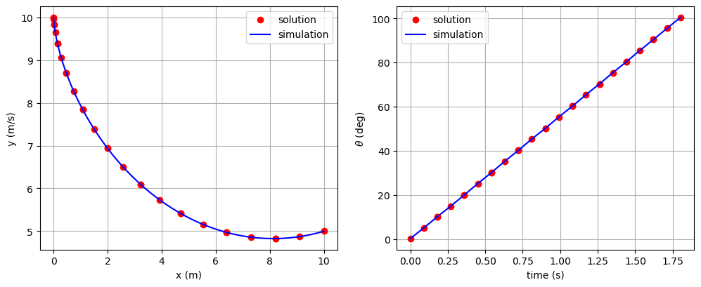
This example is the same as the other brachistochrone example with one exception: the control values come from an external source upstream of the trajectory.
The following script fully defines the brachistochrone problem with Dymos and solves it.
A new IndepVarComp is added before the trajectory.
The transcription used in the relevant phase is defined first so that we can obtain the number of control input nodes.
The IndepVarComp then provides the control \(\theta\) at the correct number of nodes, and sends them to the trajectory.
Since the control values are no longer managed by Dymos, they are added as design variables using the OpenMDAO add_design_var method.
import numpy as np
import openmdao.api as om
import dymos as dm

import matplotlib.pyplot as plt
from dymos.examples.brachistochrone.brachistochrone_ode import BrachistochroneODE

#
# Define the OpenMDAO problem
#
p = om.Problem(model=om.Group())

# Instantiate the transcription so we can get the number of nodes from it while
# building the problem.
tx = dm.GaussLobatto(num_segments=10, order=3)

# Add an indep var comp to provide the external control values
ivc = p.model.add_subsystem('control_ivc', om.IndepVarComp(), promotes_outputs=['*'])

# Add the output to provide the values of theta at the control input nodes of the transcription.
ivc.add_output('theta', shape=(tx.grid_data.subset_num_nodes['control_input']), units='rad')

# Add this external control as a design variable
p.model.add_design_var('theta', units='rad', lower=1.0E-5, upper=np.pi)
# Connect this to controls:theta in the appropriate phase.
# connect calls are cached, so we can do this before we actually add the trajectory to the problem.
p.model.connect('theta', 'traj.phase0.controls:theta')

#
# Define a Trajectory object
#
traj = dm.Trajectory()

p.model.add_subsystem('traj', subsys=traj)

#
# Define a Dymos Phase object with GaussLobatto Transcription
#
phase = dm.Phase(ode_class=BrachistochroneODE,
                 transcription=tx)

traj.add_phase(name='phase0', phase=phase)

#
# Set the time options
# Time has no targets in our ODE.
# We fix the initial time so that the it is not a design variable in the optimization.
# The duration of the phase is allowed to be optimized, but is bounded on [0.5, 10].
#
phase.set_time_options(fix_initial=True, duration_bounds=(0.5, 10.0), units='s')

#
# Set the time options
# Initial values of positions and velocity are all fixed.
# The final value of position are fixed, but the final velocity is a free variable.
# The equations of motion are not functions of position, so 'x' and 'y' have no targets.
# The rate source points to the output in the ODE which provides the time derivative of the
# given state.
phase.add_state('x', fix_initial=True, fix_final=True, units='m', rate_source='xdot')
phase.add_state('y', fix_initial=True, fix_final=True, units='m', rate_source='ydot')
phase.add_state('v', fix_initial=True, fix_final=False, units='m/s',
                rate_source='vdot', targets=['v'])

# Define theta as a control.
# Use opt=False to allow it to be connected to an external source.
# Arguments lower and upper are no longer valid for an input control.
phase.add_control(name='theta', targets=['theta'], opt=False)

# Minimize final time.
phase.add_objective('time', loc='final')

# Set the driver.
p.driver = om.ScipyOptimizeDriver()

# Allow OpenMDAO to automatically determine our sparsity pattern.
# Doing so can significant speed up the execution of Dymos.
p.driver.declare_coloring()

# Setup the problem
p.setup(check=True)

# Now that the OpenMDAO problem is setup, we can set the values of the states and controls.
phase.set_state_val('x', [0, 10])

phase.set_state_val('y', [10, 5])

phase.set_state_val('v', [0, 5])

phase.set_control_val('theta', [90, 90.5], units='deg')

# Run the driver to solve the problem
p.run_driver()

# Test the results
print(p.get_val('traj.phase0.timeseries.time')[-1])

# Check the validity of our results.
sim_out = traj.simulate()

# Plot the results
fig, axes = plt.subplots(nrows=1, ncols=2, figsize=(12, 4.5))

axes[0].plot(p.get_val('traj.phase0.timeseries.x'),
             p.get_val('traj.phase0.timeseries.y'),
             'ro', label='solution')

axes[0].plot(sim_out.get_val('traj.phase0.timeseries.x'),
             sim_out.get_val('traj.phase0.timeseries.y'),
             'b-', label='simulation')

axes[0].set_xlabel('x (m)')
axes[0].set_ylabel('y (m/s)')
axes[0].legend()
axes[0].grid()

axes[1].plot(p.get_val('traj.phase0.timeseries.time'),
             p.get_val('traj.phase0.timeseries.theta', units='deg'),
             'ro', label='solution')

axes[1].plot(sim_out.get_val('traj.phase0.timeseries.time'),
             sim_out.get_val('traj.phase0.timeseries.theta', units='deg'),
             'b-', label='simulation')

axes[1].set_xlabel('time (s)')
axes[1].set_ylabel(r'$\theta$ (deg)')
axes[1].legend()
axes[1].grid()

plt.show()
INFO: checking out_of_order...
INFO: out_of_order check complete (0.000314 sec).
INFO: checking system...
INFO: system check complete (0.000021 sec).
INFO: checking solvers...
INFO: solvers check complete (0.000172 sec).
INFO: checking dup_inputs...
INFO: dup_inputs check complete (0.000093 sec).
INFO: checking missing_recorders...
WARNING: The Problem has no recorder of any kind attached
INFO: missing_recorders check complete (0.000464 sec).
INFO: checking unserializable_options...
INFO: unserializable_options check complete (0.001127 sec).
INFO: checking comp_has_no_outputs...
INFO: comp_has_no_outputs check complete (0.000041 sec).
INFO: checking auto_ivc_warnings...
INFO: auto_ivc_warnings check complete (0.000003 sec).
Jacobian shape: (31, 50)  (13.81% nonzero)
FWD solves: 8   REV solves: 0
Total colors vs. total size: 8 vs 50  (84.00% improvement)

Sparsity computed using tolerance: 1e-25.
Dense total jacobian for Problem 'problem' was computed 3 times.
Time to compute sparsity:   0.0554 sec
Time to compute coloring:   0.0332 sec
Memory to compute coloring:   0.2773 MB
Coloring created on: 2026-03-03 15:57:16
Optimization terminated successfully    (Exit mode 0)
            Current function value: 1.8016045435421981
            Iterations: 45
            Function evaluations: 54
            Gradient evaluations: 45
Optimization Complete
-----------------------------------
[1.80160454]

Simulating trajectory traj
Done simulating trajectory traj


