The Brachistochrone with externally-sourced initial state values#
Things you’ll learn through this example
How to link phase initial time and duration.
This is another modification of the brachistochrone in which the target initial time and duration of a phase is provided by an external source (an IndepVarComp in this case).
Rather than the external value being directly connected to the phase, the values are “linked” via state_ivc’s t_initial and t_duration.
The following script fully defines the brachistochrone problem with Dymos and solves it. A new IndepVarComp is added before the trajectory which provides t_initial and t_duration. These two outputs are connected directly into the phase. Also, it’s important to set input_duration and input_initial to True inside of set_time_options
import openmdao.api as om
import dymos as dm
import matplotlib.pyplot as plt
from dymos.examples.brachistochrone.brachistochrone_ode import BrachistochroneODE
#
# Define the OpenMDAO problem
#
p = om.Problem(model=om.Group())

# Instantiate the transcription so we can get the number of nodes from it while
# building the problem.
tx = dm.GaussLobatto(num_segments=10, order=3)

# Add an indep var comp to provide the external control values
ivc = p.model.add_subsystem('states_ivc', om.IndepVarComp(), promotes_outputs=['*'])

# Add the output to provide the values of theta at the control input nodes of the transcription.
# ivc.add_output('x0', shape=(1,), units='m')
ivc.add_output('t_initial', val=0.0, units='s')
ivc.add_output('t_duration', val=10., units='s')
ivc.add_design_var('t_duration', units='s', lower=0.1, upper=10.)

# Connect x0 to the state error component so we can constrain the given value of x0
# to be equal to the value chosen in the phase.
# p.model.connect('x0', 'state_error_comp.x0_target')
# p.model.connect('traj.phase0.timeseries.x', 'state_error_comp.x0_actual',
#                 src_indices=[0])
p.model.connect('t_initial', 'traj.phase0.t_initial')
p.model.connect('t_duration', 'traj.phase0.t_duration')
#
# Define a Trajectory object
#
traj = dm.Trajectory()
p.model.add_subsystem('traj', subsys=traj)

#
# Define a Dymos Phase object with GaussLobatto Transcription
#
phase = dm.Phase(ode_class=BrachistochroneODE,
                 transcription=tx)
traj.add_phase(name='phase0', phase=phase)

#
# Set the time options
# Time has no targets in our ODE.
# We fix the initial time so that the it is not a design variable in the optimization.
# The duration of the phase is allowed to be optimized, but is bounded on [0.5, 10]
# which is set above in state_ivc
phase.set_time_options(input_duration=True, input_initial=True, units='s')

#
# Set the time options
# Initial values of positions and velocity are all fixed.
# The final value of position are fixed, but the final velocity is a free variable.
# The equations of motion are not functions of position, so 'x' and 'y' have no targets.
# The rate source points to the output in the ODE which provides the time derivative of the
# given state.
phase.add_state('x', fix_initial=True, fix_final=True, units='m', rate_source='xdot')
phase.add_state('y', fix_initial=True, fix_final=True, units='m', rate_source='ydot')
phase.add_state('v', fix_initial=True, fix_final=False, units='m/s',
                rate_source='vdot', targets=['v'])

# Define theta as a control.
# Use opt=False to allow it to be connected to an external source.
# Arguments lower and upper are no longer valid for an input control.
phase.add_control(name='theta', units='rad', targets=['theta'])
# Minimize final time.
phase.add_objective('time', loc='final')

# Set the driver.
p.driver = om.ScipyOptimizeDriver()

# Allow OpenMDAO to automatically determine our sparsity pattern.
# Doing so can significant speed up the execution of Dymos.
p.driver.declare_coloring()

# Setup the problem
p.setup(check=True)

# Now that the OpenMDAO problem is setup, we can set the values of the states.
# p.set_val('x0', 0.0, units='m')
# Here we're intentially setting the intiial x value to something other than zero, just
# to demonstrate that the optimizer brings it back in line with the value of x0 set above.
p.set_val('traj.phase0.states:x',
          phase.interp('x', [0, 10]),
          units='m')
p.set_val('traj.phase0.states:y',
          phase.interp('y', [10, 5]),
          units='m')
p.set_val('traj.phase0.states:v',
          phase.interp('v', [0, 5]),
          units='m/s')
p.set_val('traj.phase0.controls:theta',
          phase.interp('theta', [90, 90]),
          units='deg')

# Run the driver to solve the problem
dm.run_problem(p, simulate=True)
--- Constraint Report [traj] ---
    --- phase0 ---
        None

INFO: checking out_of_order
/usr/share/miniconda/envs/test/lib/python3.10/site-packages/openmdao/recorders/sqlite_recorder.py:227: UserWarning:The existing case recorder file, dymos_solution.db, is being overwritten.
INFO:check_config:checking out_of_order
INFO: checking system
INFO:check_config:checking system
INFO: checking solvers
INFO:check_config:checking solvers
INFO: checking dup_inputs
INFO:check_config:checking dup_inputs
INFO: checking missing_recorders
INFO:check_config:checking missing_recorders
WARNING: The Problem has no recorder of any kind attached
WARNING:check_config:The Problem has no recorder of any kind attached
INFO: checking unserializable_options
INFO:check_config:checking unserializable_options
INFO: checking comp_has_no_outputs
INFO:check_config:checking comp_has_no_outputs
INFO: checking auto_ivc_warnings
INFO:check_config:checking auto_ivc_warnings
Model viewer data has already been recorded for Driver.
INFO: checking out_of_order
INFO:check_config:checking out_of_order
INFO: checking system
INFO:check_config:checking system
INFO: checking solvers
INFO:check_config:checking solvers
INFO: checking dup_inputs
INFO:check_config:checking dup_inputs
INFO: checking missing_recorders
INFO:check_config:checking missing_recorders
WARNING: The Problem has no recorder of any kind attached
WARNING:check_config:The Problem has no recorder of any kind attached
INFO: checking unserializable_options
INFO:check_config:checking unserializable_options
INFO: checking comp_has_no_outputs
INFO:check_config:checking comp_has_no_outputs
INFO: checking auto_ivc_warnings
INFO:check_config:checking auto_ivc_warnings
Full total jacobian was computed 3 times, taking 0.177579 seconds.
Total jacobian shape: (40, 50)


Jacobian shape: (40, 50)  (13.40% nonzero)
FWD solves: 8   REV solves: 0
Total colors vs. total size: 8 vs 50  (84.0% improvement)

Sparsity computed using tolerance: 1e-25
Time to compute sparsity: 0.177579 sec.
Time to compute coloring: 0.049746 sec.
Memory to compute coloring: 0.375000 MB.
Optimization terminated successfully    (Exit mode 0)
            Current function value: [1.80160435]
            Iterations: 60
            Function evaluations: 62
            Gradient evaluations: 60
Optimization Complete
-----------------------------------
Simulating trajectory traj
Model viewer data has already been recorded for Driver.
Done simulating trajectory traj
False
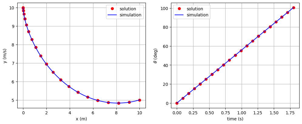
Plotting the results#
In the following cell, we load the solution and simulated results from their respective recorder files and plot the solution.
# Check the validity of our results by using scipy.integrate.solve_ivp to
# integrate the solution.
sol = om.CaseReader('dymos_solution.db').get_case('final')
sim = om.CaseReader('dymos_simulation.db').get_case('final')

# Plot the results
fig, axes = plt.subplots(nrows=1, ncols=2, figsize=(12, 4.5))
axes[0].plot(sol.get_val('traj.phase0.timeseries.x'),
             sol.get_val('traj.phase0.timeseries.y'),
             'ro', label='solution')
axes[0].plot(sim.get_val('traj.phase0.timeseries.x'),
             sim.get_val('traj.phase0.timeseries.y'),
             'b-', label='simulation')
axes[0].set_xlabel('x (m)')
axes[0].set_ylabel('y (m/s)')
axes[0].legend()
axes[0].grid()
axes[1].plot(sol.get_val('traj.phase0.timeseries.time'),
             sol.get_val('traj.phase0.timeseries.theta', units='deg'),
             'ro', label='solution')
axes[1].plot(sim.get_val('traj.phase0.timeseries.time'),
             sim.get_val('traj.phase0.timeseries.theta', units='deg'),
             'b-', label='simulation')
axes[1].set_xlabel('time (s)')
axes[1].set_ylabel(r'$\theta$ (deg)')
axes[1].legend()
axes[1].grid()
plt.show()