The Brachistochrone with externally-sourced initial state values#
Things you’ll learn through this example
How to link phase initial time and duration.
This is another modification of the brachistochrone in which the target initial time and duration of a phase is provided by an external source (an IndepVarComp in this case).
Rather than the external value being directly connected to the phase, the values are “linked” via state_ivc’s t_initial and t_duration.
The following script fully defines the brachistochrone problem with Dymos and solves it. A new IndepVarComp is added before the trajectory which provides t_initial and t_duration. These two outputs are connected directly into the phase. Also, it’s important to set input_duration and input_initial to True inside of set_time_options
import openmdao.api as om
import dymos as dm
import matplotlib.pyplot as plt
from dymos.examples.brachistochrone.brachistochrone_ode import BrachistochroneODE
#
# Define the OpenMDAO problem
#
p = om.Problem(model=om.Group())

# Instantiate the transcription so we can get the number of nodes from it while
# building the problem.
tx = dm.GaussLobatto(num_segments=10, order=3)

# Add an indep var comp to provide the external control values
ivc = p.model.add_subsystem('states_ivc', om.IndepVarComp(), promotes_outputs=['*'])

# Add the output to provide the values of theta at the control input nodes of the transcription.
# ivc.add_output('x0', shape=(1,), units='m')
ivc.add_output('t_initial', val=0.0, units='s')
ivc.add_output('t_duration', val=10., units='s')
ivc.add_design_var('t_duration', units='s', lower=0.1, upper=10.)

# Connect x0 to the state error component so we can constrain the given value of x0
# to be equal to the value chosen in the phase.
# p.model.connect('x0', 'state_error_comp.x0_target')
# p.model.connect('traj.phase0.timeseries.x', 'state_error_comp.x0_actual',
#                 src_indices=[0])
p.model.connect('t_initial', 'traj.phase0.t_initial')
p.model.connect('t_duration', 'traj.phase0.t_duration')
#
# Define a Trajectory object
#
traj = dm.Trajectory()
p.model.add_subsystem('traj', subsys=traj)

#
# Define a Dymos Phase object with GaussLobatto Transcription
#
phase = dm.Phase(ode_class=BrachistochroneODE,
                 transcription=tx)
traj.add_phase(name='phase0', phase=phase)

#
# Set the time options
# Time has no targets in our ODE.
# We fix the initial time so that the it is not a design variable in the optimization.
# The duration of the phase is allowed to be optimized, but is bounded on [0.5, 10]
# which is set above in state_ivc
phase.set_time_options(input_duration=True, input_initial=True, units='s')

#
# Set the time options
# Initial values of positions and velocity are all fixed.
# The final value of position are fixed, but the final velocity is a free variable.
# The equations of motion are not functions of position, so 'x' and 'y' have no targets.
# The rate source points to the output in the ODE which provides the time derivative of the
# given state.
phase.add_state('x', fix_initial=True, fix_final=True, units='m', rate_source='xdot')
phase.add_state('y', fix_initial=True, fix_final=True, units='m', rate_source='ydot')
phase.add_state('v', fix_initial=True, fix_final=False, units='m/s',
                rate_source='vdot', targets=['v'])

# Define theta as a control.
# Use opt=False to allow it to be connected to an external source.
# Arguments lower and upper are no longer valid for an input control.
phase.add_control(name='theta', units='rad', targets=['theta'])
# Minimize final time.
phase.add_objective('time', loc='final')

# Set the driver.
p.driver = om.ScipyOptimizeDriver()

# Allow OpenMDAO to automatically determine our sparsity pattern.
# Doing so can significant speed up the execution of Dymos.
p.driver.declare_coloring()

# Setup the problem
p.setup(check=True)

# Now that the OpenMDAO problem is setup, we can set the values of the states.
# p.set_val('x0', 0.0, units='m')
# Here we're intentially setting the intiial x value to something other than zero, just
# to demonstrate that the optimizer brings it back in line with the value of x0 set above.
phase.set_state_val('x', [0, 10],
                    units='m')

phase.set_state_val('y', [10, 5],
                    units='m')

phase.set_state_val('v', [0, 9.9],
                    units='m/s')

phase.set_control_val('theta', [5, 100.5],
                      units='deg')

# Run the driver to solve the problem
dm.run_problem(p, simulate=True)
--- Constraint Report [traj] ---
    --- phase0 ---
        None

INFO: checking out_of_order
INFO: checking system
INFO: checking solvers
INFO: checking dup_inputs
INFO: checking missing_recorders
INFO: checking unserializable_options
INFO: checking comp_has_no_outputs
INFO: checking auto_ivc_warnings
Model viewer data has already been recorded for Driver.
INFO: checking out_of_order
INFO: checking system
INFO: checking solvers
INFO: checking dup_inputs
INFO: checking missing_recorders
INFO: checking unserializable_options
INFO: checking comp_has_no_outputs
INFO: checking auto_ivc_warnings
/usr/share/miniconda/envs/test/lib/python3.11/site-packages/openmdao/recorders/sqlite_recorder.py:231: UserWarning:The existing case recorder file, /home/runner/work/dymos/dymos/docs/dymos_book/examples/brachistochrone/problem_out/dymos_solution.db, is being overwritten.
Full total jacobian for problem 'problem' was computed 3 times, taking 0.07827906299996812 seconds.
Total jacobian shape: (40, 50)


Jacobian shape: (40, 50)  (13.40% nonzero)
FWD solves: 8   REV solves: 0
Total colors vs. total size: 8 vs 50  (84.00% improvement)

Sparsity computed using tolerance: 1e-25
Time to compute sparsity:   0.0783 sec
Time to compute coloring:   0.0223 sec
Memory to compute coloring:   0.1250 MB
Coloring created on: 2024-10-02 16:46:21
Optimization terminated successfully    (Exit mode 0)
            Current function value: 1.8016052392021373
            Iterations: 39
            Function evaluations: 40
            Gradient evaluations: 39
Optimization Complete
-----------------------------------
/usr/share/miniconda/envs/test/lib/python3.11/site-packages/openmdao/core/group.py:1137: DerivativesWarning:Constraints or objectives [ode_eval.control_interp.control_rates:theta_rate, ode_eval.control_interp.control_rates:theta_rate2, ode_eval.control_interp.control_values:theta] cannot be impacted by the design variables of the problem because no partials were defined for them in their parent component(s).
Simulating trajectory traj
Model viewer data has already been recorded for Driver.
Done simulating trajectory traj
Problem: problem
Driver:  ScipyOptimizeDriver
  success     : True
  iterations  : 41
  runtime     : 6.8964E-01 s
  model_evals : 41
  model_time  : 2.7786E-02 s
  deriv_evals : 39
  deriv_time  : 2.0372E-01 s
  exit_status : SUCCESS
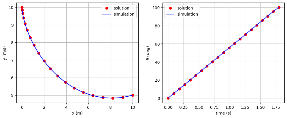
Plotting the results#
In the following cell, we load the solution and simulated results from their respective recorder files and plot the solution.
# Check the validity of our results.
sol = om.CaseReader(p.get_outputs_dir() / 'dymos_solution.db').get_case('final')
sim = om.CaseReader(traj.sim_prob.get_outputs_dir() / 'dymos_simulation.db').get_case('final')

# Plot the results
fig, axes = plt.subplots(nrows=1, ncols=2, figsize=(12, 4.5))
axes[0].plot(sol.get_val('traj.phase0.timeseries.x'),
             sol.get_val('traj.phase0.timeseries.y'),
             'ro', label='solution')
axes[0].plot(sim.get_val('traj.phase0.timeseries.x'),
             sim.get_val('traj.phase0.timeseries.y'),
             'b-', label='simulation')
axes[0].set_xlabel('x (m)')
axes[0].set_ylabel('y (m/s)')
axes[0].legend()
axes[0].grid()
axes[1].plot(sol.get_val('traj.phase0.timeseries.time'),
             sol.get_val('traj.phase0.timeseries.theta', units='deg'),
             'ro', label='solution')
axes[1].plot(sim.get_val('traj.phase0.timeseries.time'),
             sim.get_val('traj.phase0.timeseries.theta', units='deg'),
             'b-', label='simulation')
axes[1].set_xlabel('time (s)')
axes[1].set_ylabel(r'$\theta$ (deg)')
axes[1].legend()
axes[1].grid()
plt.show()


